Pixel Classification

Pixel Classification Demo (3 minutes)

How it works, what it can do

The Pixel Classification workflow assigns labels to pixels based on pixel features and user annotations. The workflow offers a choice of generic pixel features, such as smoothed pixel intensity, edge filters and texture descriptors. Once the features are selected, a Random Forest classifier is trained from user annotations interactively. The Random Forest is known for its excellent generalization properties, the overall workflow is applicable to a wide range of segmentation problems. Note that this workflow performs semantic, rather than instance, segmentation and returns a probability map of each class, not individual objects. The probability map can be transformed into individual objects by a variety of methods. The simplest is, perhaps, thresholding and connected component analysis which is provided in the ilastik Object Classification Workflow. Other alternatives include more sophisticated thresholding, watershed and agglomeration algorithms in Fiji and other popular image analysis tools.

In order to follow this tutorial, you can download the used example project here. Used image data is courtesy of Daniel Gerlich.

A typical cell segmentation use case is depicted below.

Nice properties of the algorithm and workflow are

• Interactive mode: the user gets immediate feedback after giving additional annotations.
• Batch mode: the trained classifier can be applied to previously unseen images. Results are written to disk.
• Uncertainty guidance: the user can view an uncertainty map, this indicates areas where the classifier is unsure about the results. Additional annotations in these regions help most.

Selecting good features

As usual, start by loading the data as described in the basics. After the data is loaded, switch to the next applet Feature Selection. Here you will select the pixel features and their scales which in the next step will be used to discriminate between the different classes of pixels.

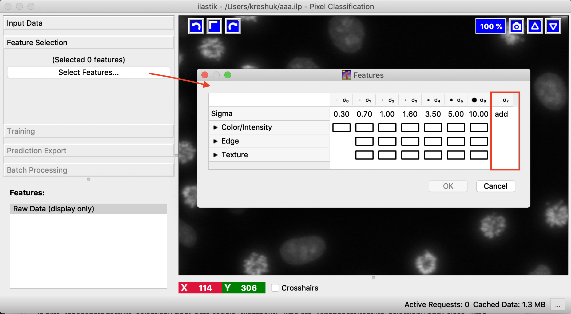
A click on the Select features button brings up a feature selection dialog.

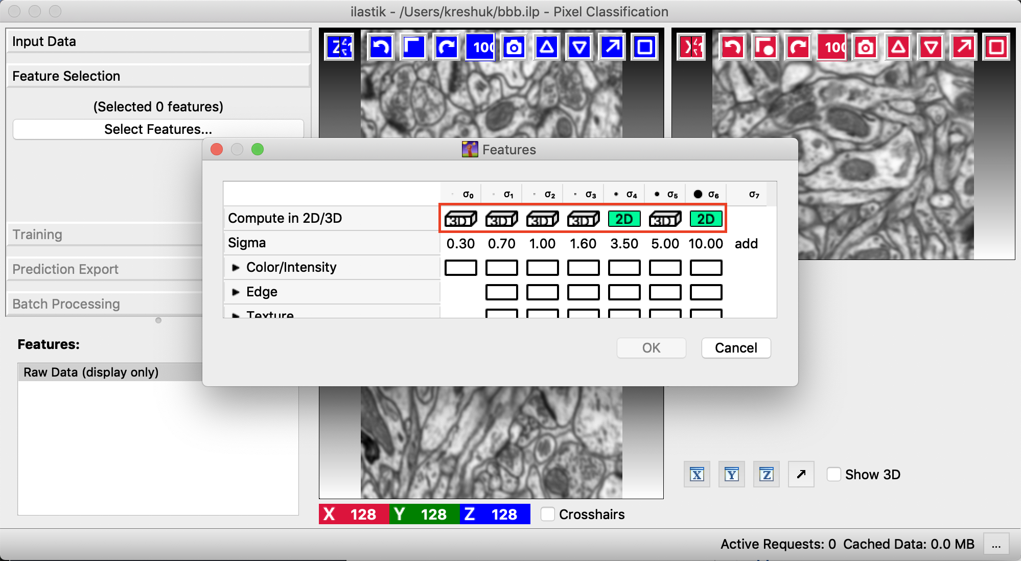
For 3D data the features can be computed either in 2D or 3D. 2D can be useful if data has thick slices and the information from a slice is not so relevant for the neighbors. It is also the only way to compute large-scale filters in thin stacks. The following image shows the switch between 2D and 3D computation in the Feature Selection dialog.

We provide the following feature types:

• Color/Intensity: these features should be selected if the color or brightness can be used to discern objects
• Edge: should be selected if brightness or color gradients can be used to discern objects.
• Texture: this might be an important feature if the objects in the image have a special textural appearance.

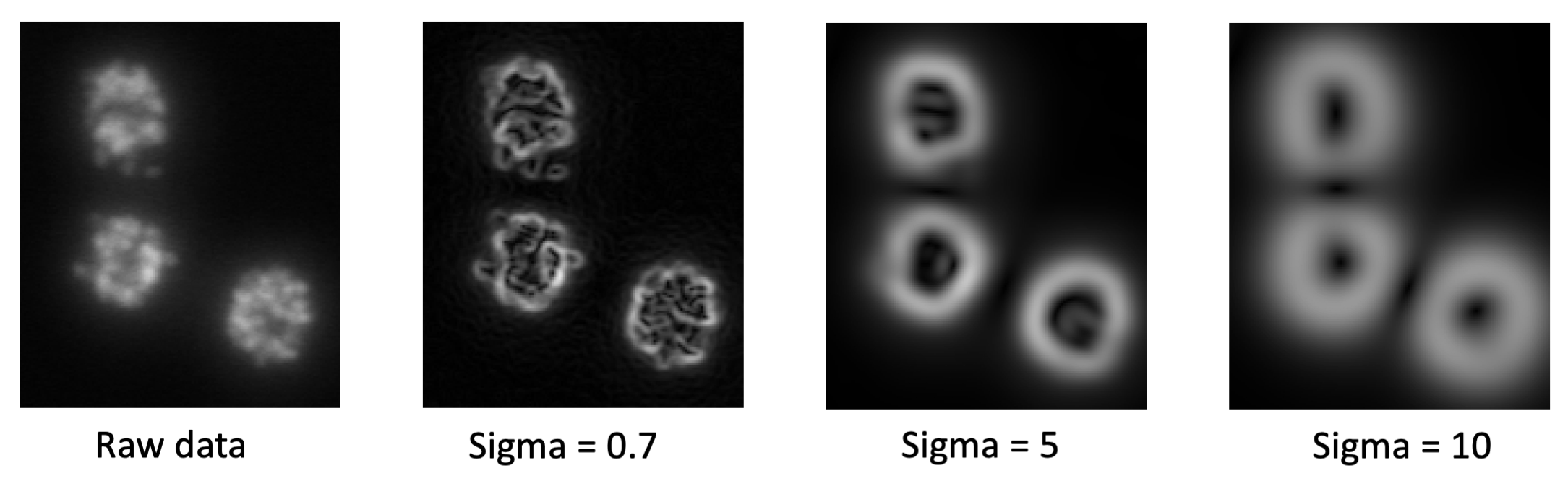
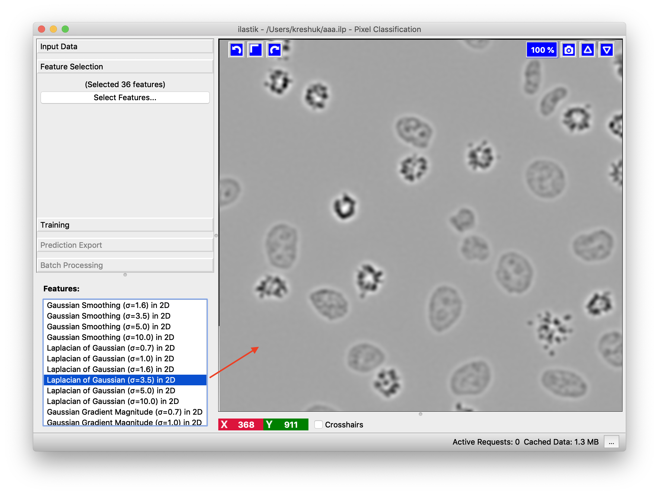
All of these features can be selected on different scales. The scales correspond to the sigma of the Gaussian which is used to smooth the image before application of the filter. Filters with larger sigmas can thus pull in information from larger neighborhoods, but average out the fine details. If you feel that a certain value of the sigma would be particularly well suited to your data, you can also add your own sigmas in the last column, as shown above in red. The following image provides an example of the edge filter computed with 3 different sigma values. Note how the filter fits to the smallest edges at the very low sigma value and only finds the rough cell outlines at a high sigma.

In general we advise to initially select a wide range of feature types and scales. In fact, for not-too-big 2D data where computation time is not a concern, one can simply select all. In the next step, after you start annotating the image, we can suggest you the most helpful features based on your labels as described here. The selected features can be inspected in the bottom left after clicking OK in the feature selection dialog.

Training the classifier

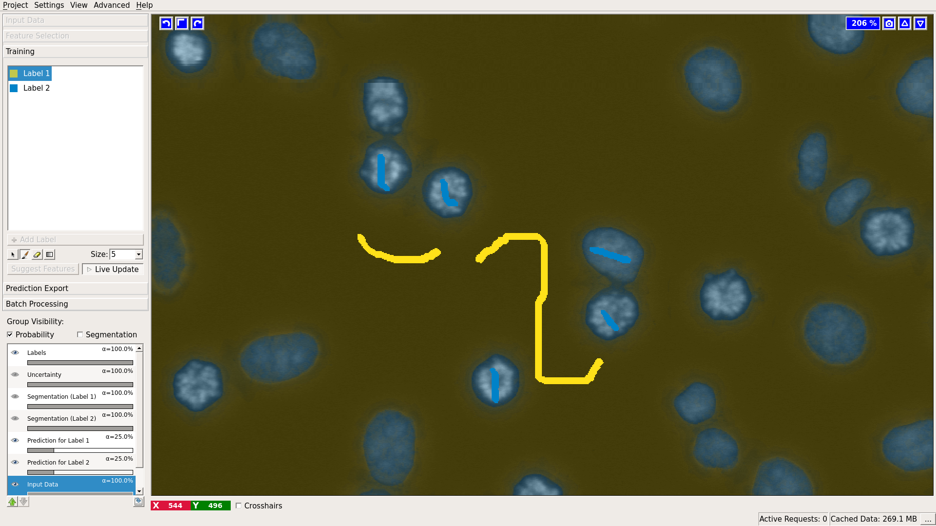
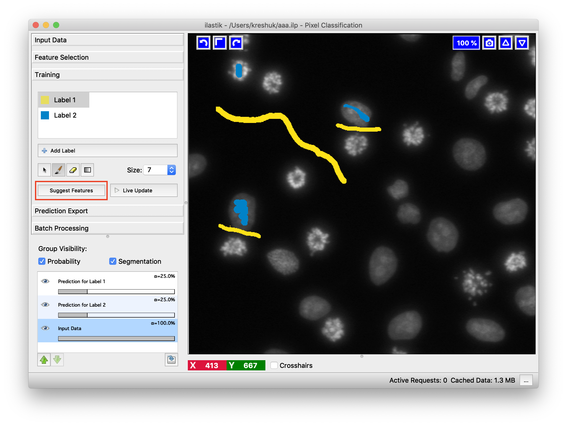
The next step in the pixel classification is the training of a classifier that can separate the object classes. This training is done in an iterative fashion, the user draws some annotations, evaluates the interactive prediction and then draws additional annotations to correct eventual mistakes. To begin with the training of the classifier, we switch to the Training applet and add some labels. 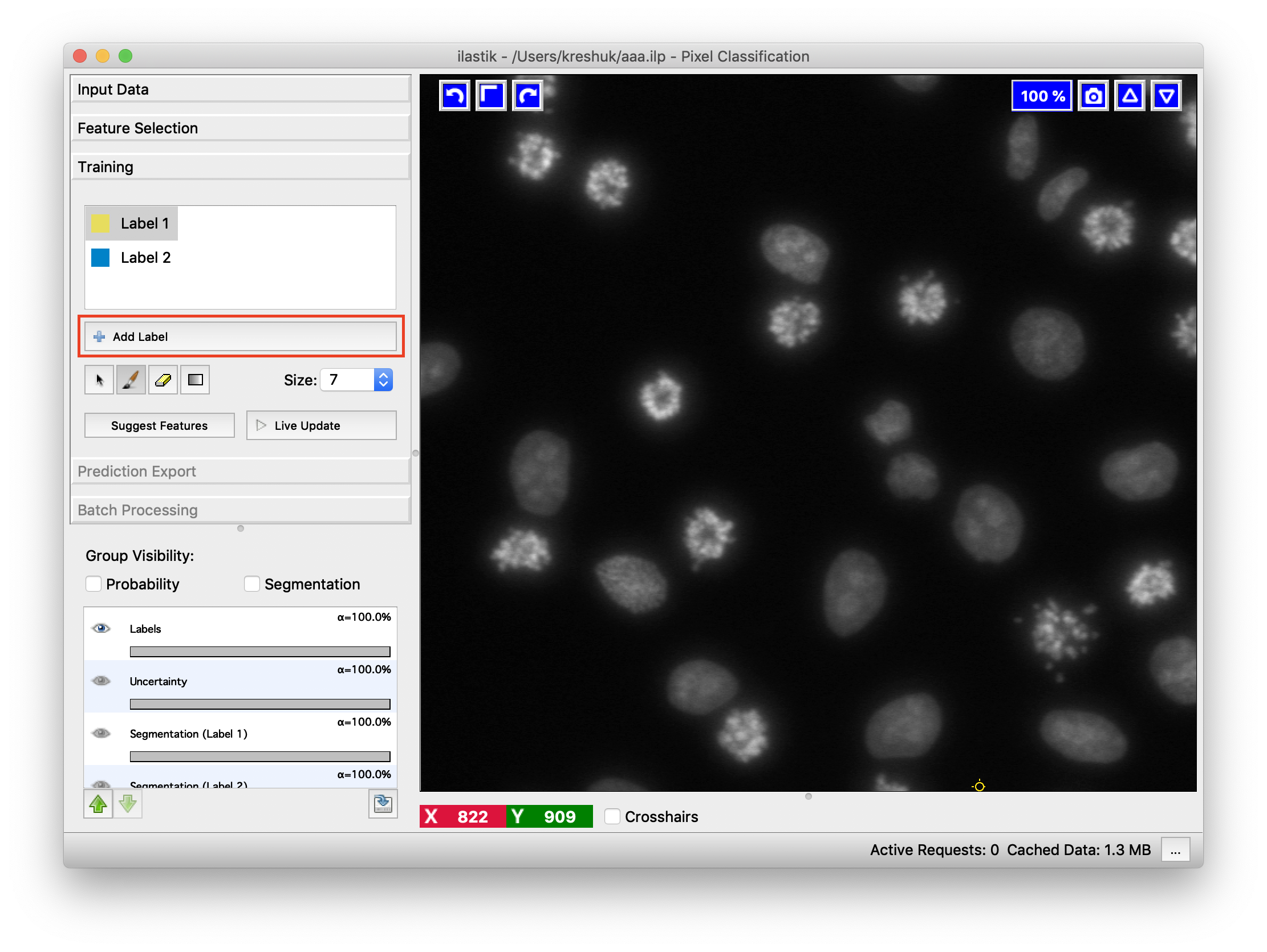Each added label should correspond to a pixel class that we want to separate. This can, for example, be “cell” and “background”, or “sky”, “grass” and “tree”. Two labels are already added by default, add more if needed by pressing the “Add Label” button. You can change the color of the annotations or the names of the labels by double-clicking on the little color square or on the “Label x” text field.

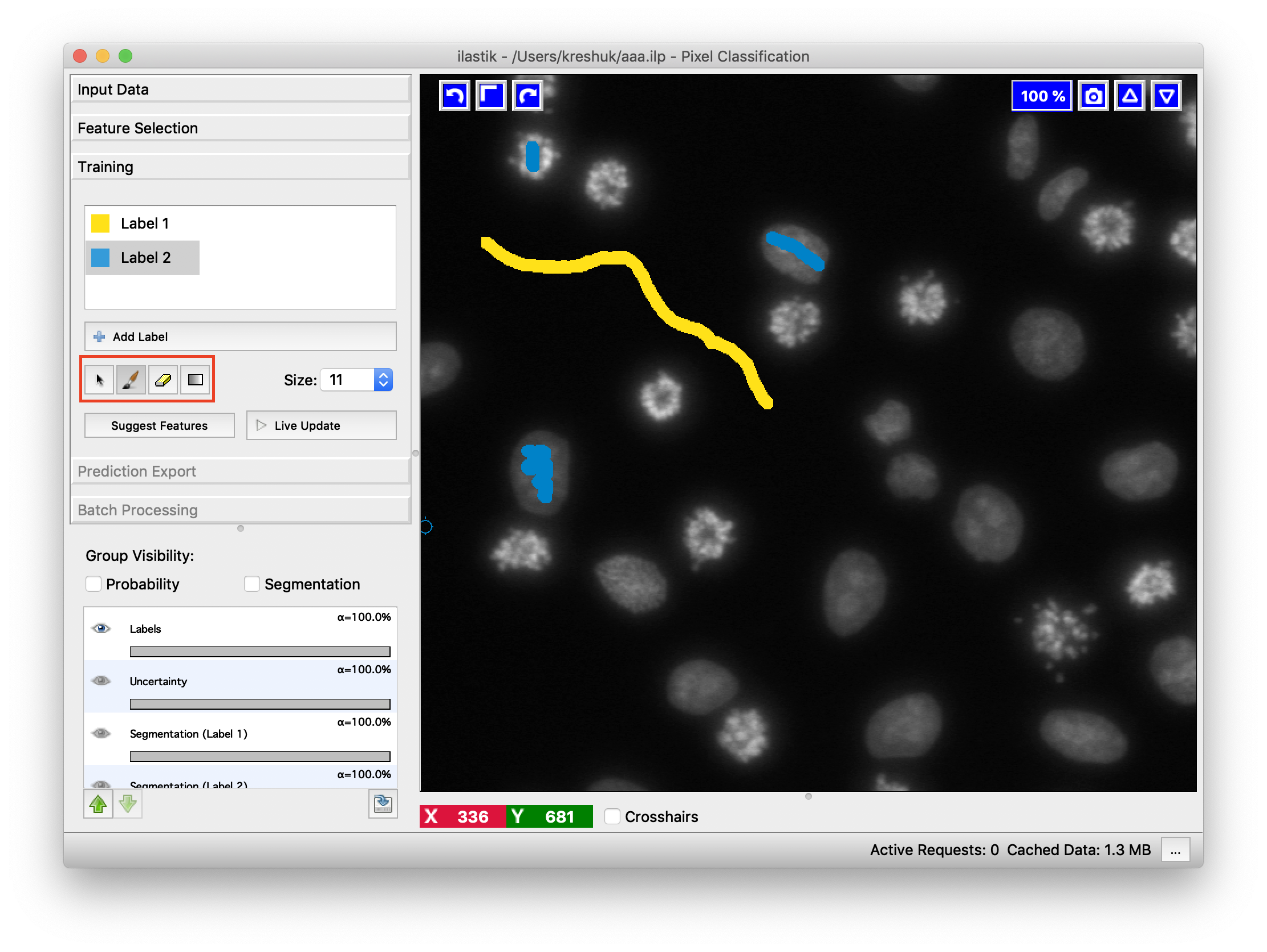
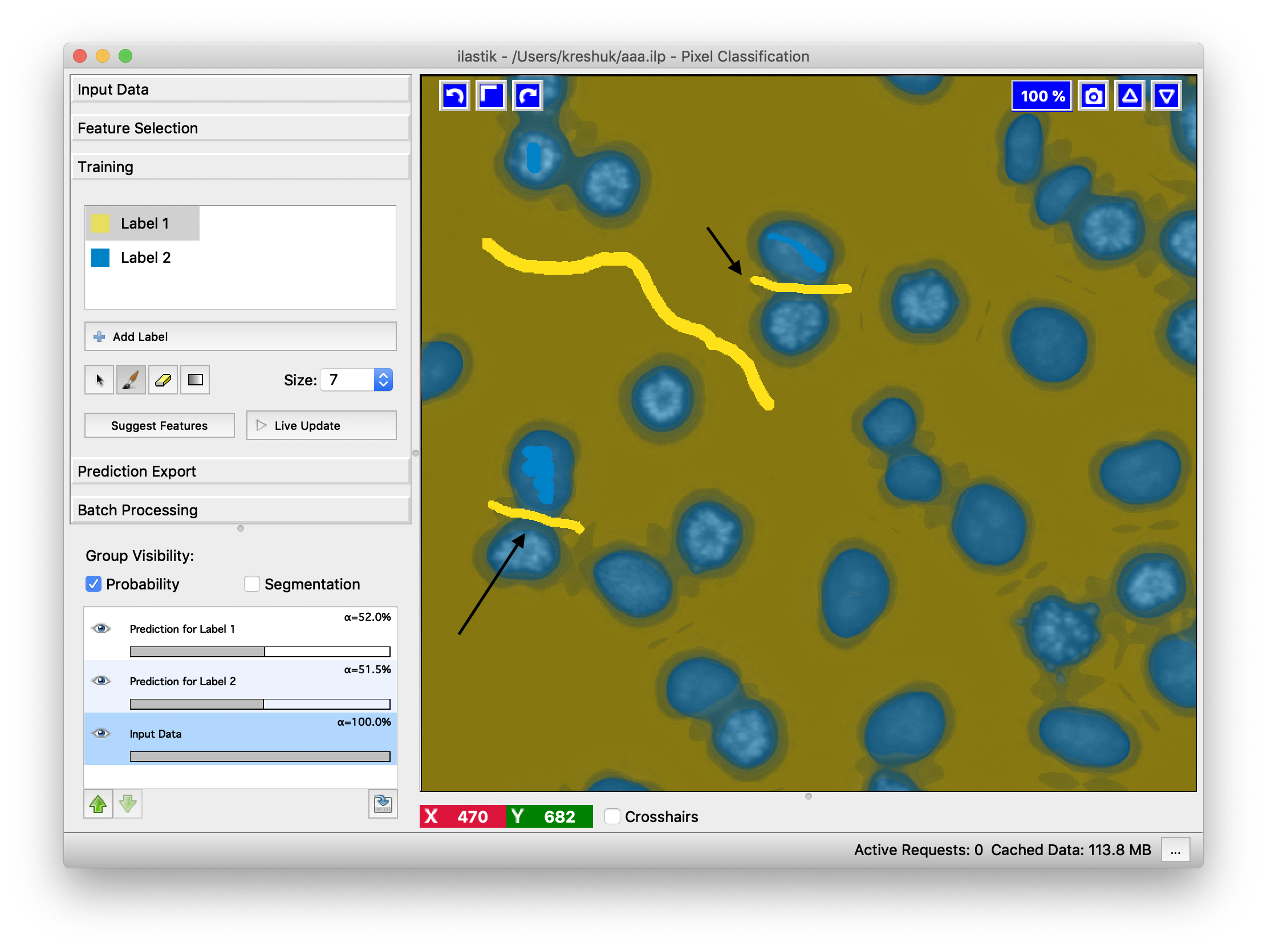
You are now ready to give some training annotations! Select a class and scribble over pixels which belong to it. Then change to another class and add more scribbles for it. If you add a wrong scribble, use an eraser to remove it (eraser controls are shown below). You can also change the size of the brush in the next control.

To train the classifier and see the predictions, press the Live update button. In the background, the features for the labeled pixels will be computed and the Random Forest classifier will be trained from your annotations. Then the features for all pixels in your field of view will be computed and their classes will be predicted by the trained classifier. The predictions will be displayed as an overlay on the image.

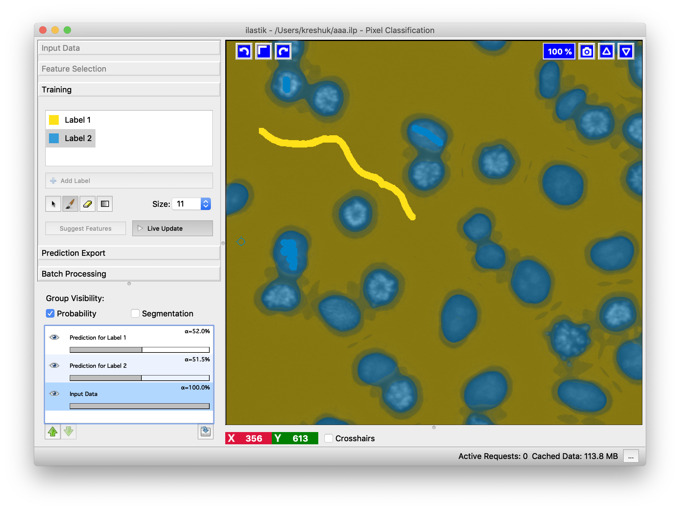
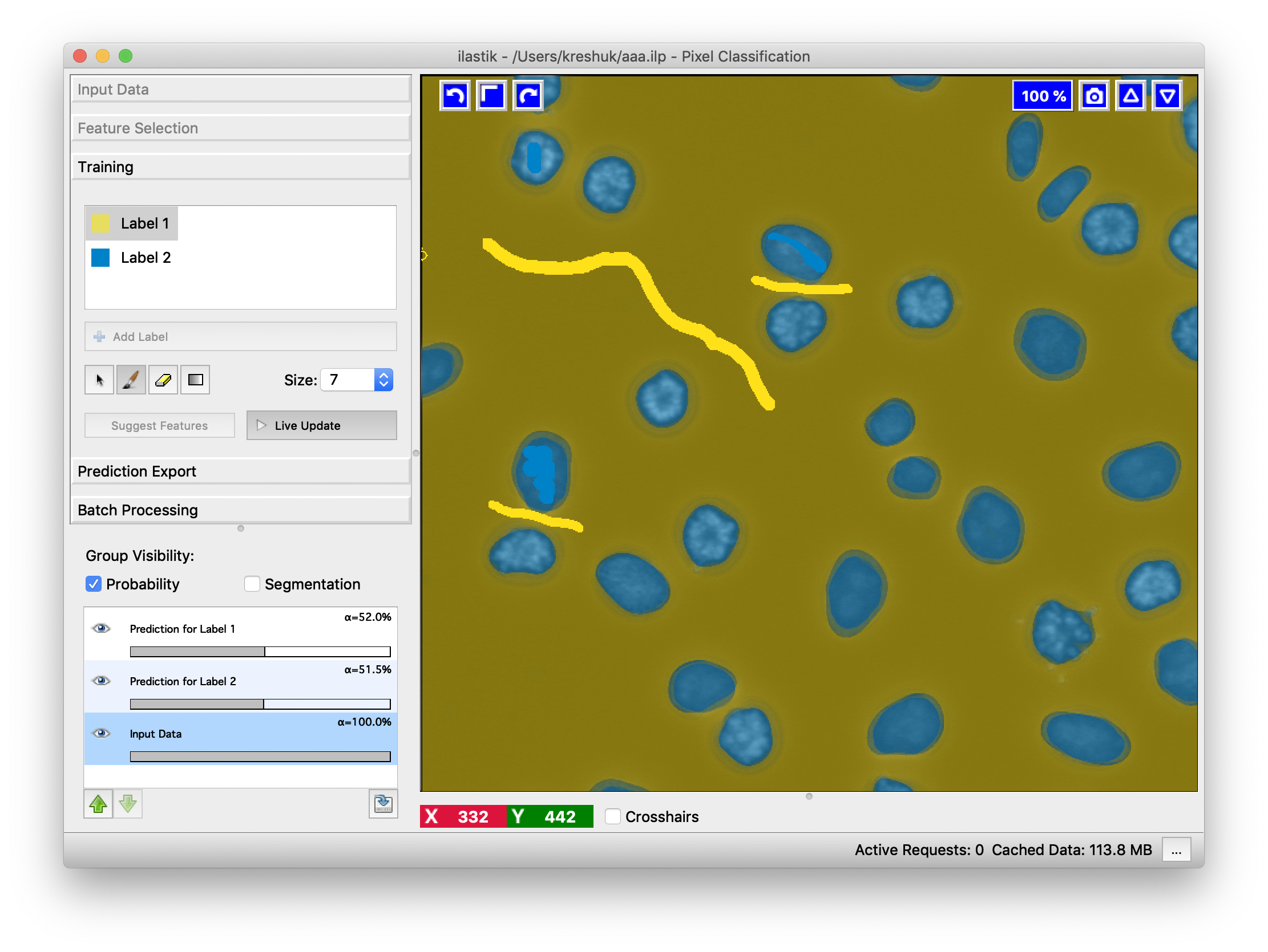
Examine the results for errors and add more annotations to correct. Here, we will add two more scribbles to separate objects which got merged in the first prediction attempt.

The classification will be updated on-the-fly. Update is much faster than the first computation since the features are cached and not recomputed. As you can see, all objects are now correctly separated. Keep introducing more annotations until you see no more errors or the predictions stops improving.

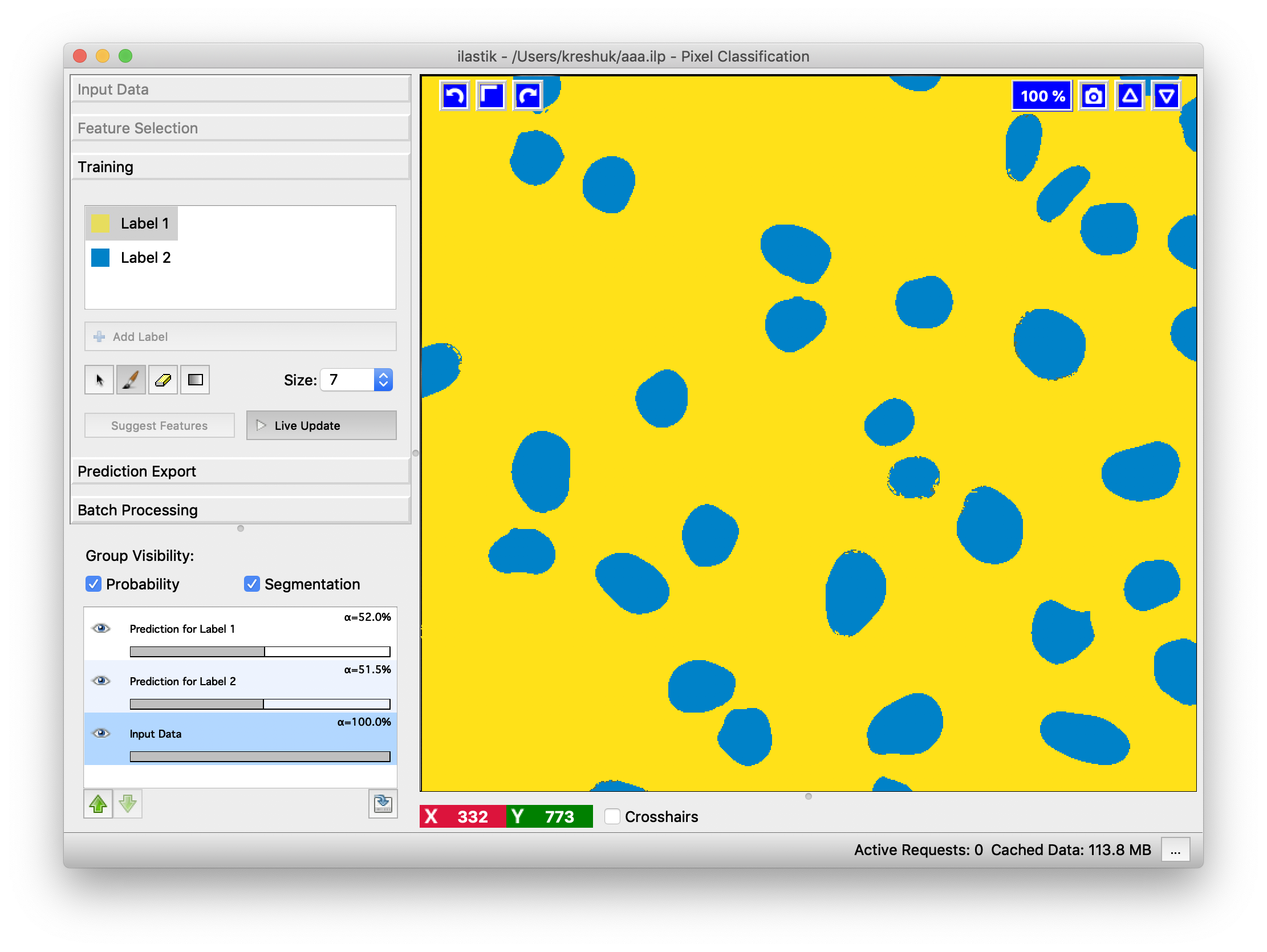
To display the hard classification results, i.e. the final class assignment the Segmentation overlays can be turned on by clicking on the Segmentation checkbox.

How to import labels from an external file

To access the “Import Labels” feature in the GUI, do the following:

1. Create N label classes (click “Add Label” N times).

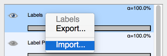
2. Right-click on the list item in the lower left-hand corner titled “Labels”. (See screenshot.) That will open up a window to allow you to import labels.

3. If your label image is the same size as your input data, and the label image pixels already have consecutive values 1..N, then the default settings may suffice. Otherwise, you can modify the settings in that window to specify how to offset the label image relative to your input data, and also how to map label image pixel values to the label values ilastik needs (1..N).

Automatic feature suggestion

If you are not confident in your choice of pixel features, Suggest Features functionality might help. Press the button and a new dialog will pop up.

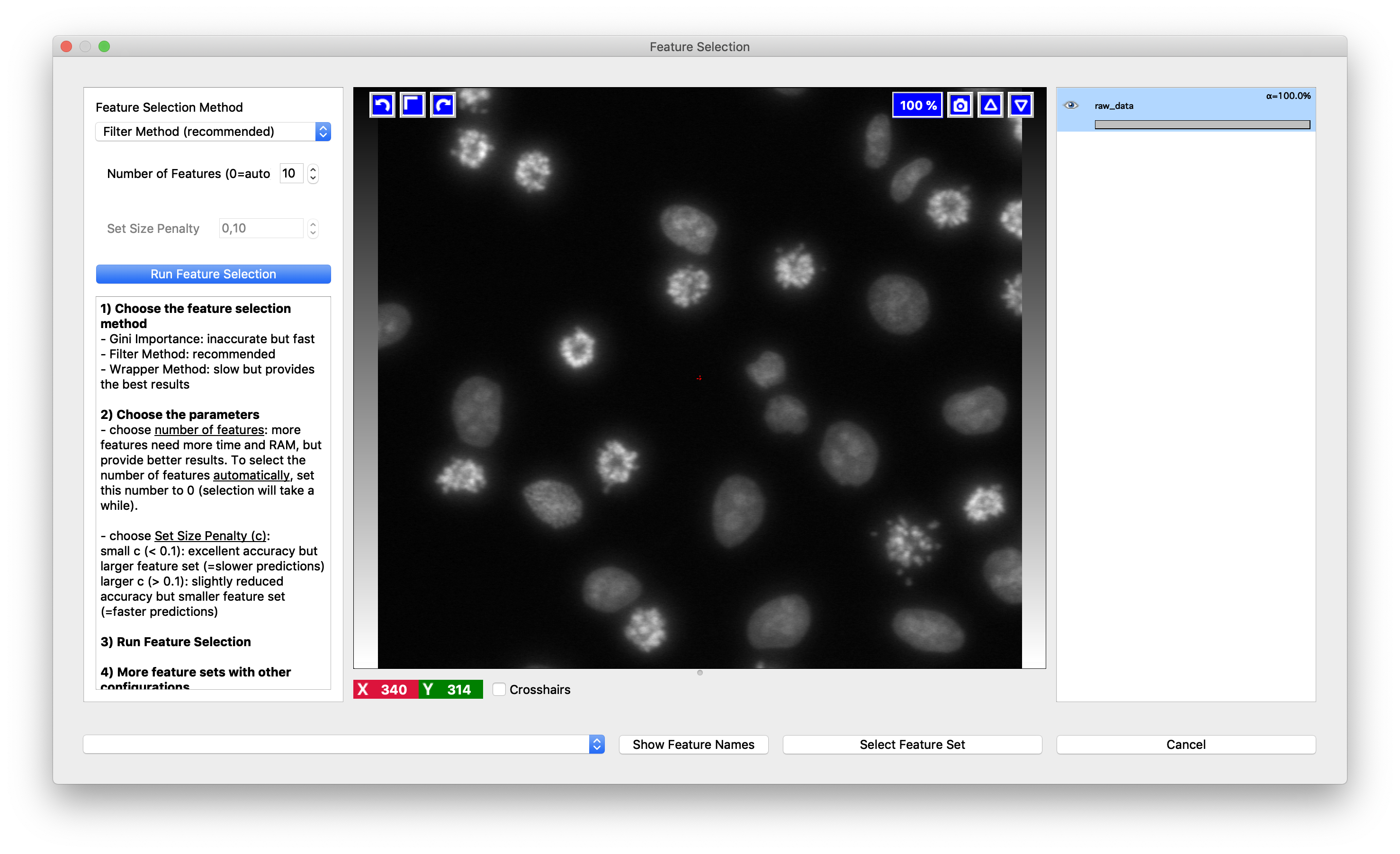
It works by evaluating the classifier predictions using different feature sets on the pixels you have already annotated. The so called “out-of-bag” predictions are used, so for every tree in the Random Forest we only use the pixels it has not seen in training to estimate the error. Still, even though the pixels were not seen in training, randomization is done on the pixel level, so the tree has likely seen some similar pixels and the error estimate is overly optimistic. Besides the error, ilastik also reports the computing time which can be helpful when trying to find the balance between runtime and accuracy. By choosing the feature set in the lower left corner, you can also see the predictions ilastik would make with these features on the current field of view.

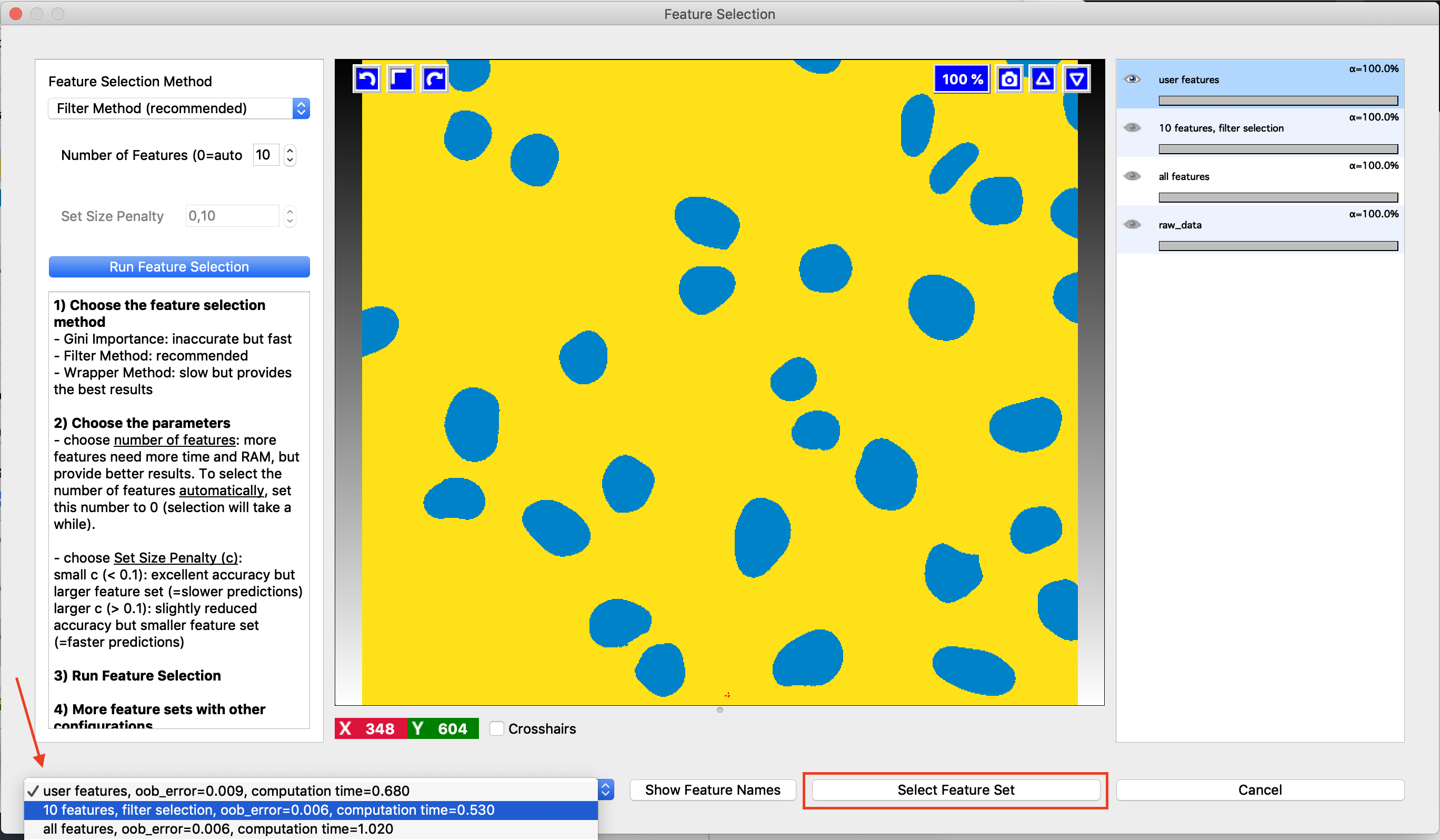
If you like one of the suggested features sets better than your current selection, you can replace your selection with the new set by pressing the Select Feature Set button.

Window Leveling

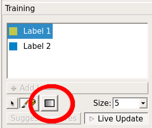If labeling grayscale images the Training applet has an additional option: Window Leveling. This option can facilitate the labeling but has no impact on the training process itself. It can be used to adjust the data range used for visualization and thus helps to bring out small difference in contrast which might be useful when placing the labels. Pressing the left mouse button while moving the mouse back and forth changes the window width (data range) used for display. Moving the mouse in the left-right plane changes the window level, i.e. the center of the window. Of course, combinations of back-forth and left-right movements are possible to find just the right contrast needed. Pressing the right mouse button leads to an automatic range adjustment based on the intensity values currently displayed. To activate this feature either press the button outlined in the image below or use its keyboard shortcut (default ‘t’).

Note: if you can not see the button, you are either not working with grayscale images or you did not set the Channel Display to Grayscale in the Dataset Properties of your Raw Data.

Processing new images in batch mode

After the classifier is trained, it can be applied to unseen images as batch processing (without further training). This follows a general procedure in ilastik and is demonstrated here.
The results of this workflow (probability maps or segmentations) can be exported as images (.tiff, .png , etc.. ) or .h5 files. Details on all export options can be found on this page. In case you select to export a probability map (this is the default), it will be saved as a multichannel image, where each channel corresponds to a class you defined during training. For example, if you are performing binary classification into foreground/background, the probability map at pixel (px, py) will have the value of the foreground probability in the first channel and the value of the background probability in the second channel. If you choose to save a simple segmentation, the result will be a label image, where pixels are assigned the value of the most probable class. For example, suppose you are performing classification with three classes and the classifier output (probability map) for pixel (px, py) is 0.3, 0.3, 0.4 for classes 0, 1, 2 respectively. In the simple segmentation image ilastik exports, pixel (px, py) will then have value 2.

Processing new images in headless mode

Actually, after the classifier is trained, you don’t need the GUI anymore. If you’d rather run without it, ilastik has a special headless mode. This can be convenient for running on a cluster or on a remote machine.