 Documentation
Interactive Segmentation
Documentation
Interactive Segmentation
Carving
Carving Demo (4 minutes)
How it works, what it can and cannot do
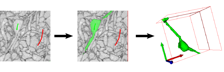
The seeded watershed algorithm is an image segmentation algorithm for interactive object extraction from image data. The algorithm input is user-defined object markers (see example below) for the inside (green) and outside (red) of an object. From these markers, an initial segmentation is calculated that can be refined interactively. The seeded watershed relies on discernible object boundaries in the image data and not on the inner appearance of an object like for example the pixel classification workflow.
While the Pixel Classification module is useful for segmenting objects with discernible brightness, color or textural differences in comparison to their surroundings, the carving module’s purpose is to aid in the extraction of objects from images that are only separable by their boundary - i.e. objects that do not differ from the rest of the image by their internal appearance.
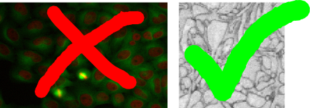
From the two example images above, the left image is clearly more suitable for the classification module since the cell cores have a strong red color component in comparison to their surrounding. The right image, on the other hand, is a good example for the applicability of the seeded watershed segmentation (the problem setting is the segmentation of a single cell from electron microscopy image of neural tissue) since the neural cells have similar color distributions but can be separated by the dark cell membranes dividing them. (NOTE: the seeded watershed could also be applied to segment individual cell cores in the left image interactively, but in such a case where there is a clear visible difference between the objects of interest and their surrounding the pixel classification module is a better choice.)
The algorithm is applicable to a wide range of segmentation problems that fulfill these properties. In the case of data where the boundaries are not clearly visible or in the case of very noisy data, a boundary detection filter can be applied to improve results - this is the topic of the following section.
Example Data: In the following sections, we use a volume of mouse retina EM data courtesy of Winfried Denk, et al.
The data can be found on the downloads page or download it directly here.
Constructing a good boundary map
Assuming the user has already created or loaded an existing ilastik project and added a dataset, the first step is to switch to the Preprocessing Applet where the filter selection and computation are performed.
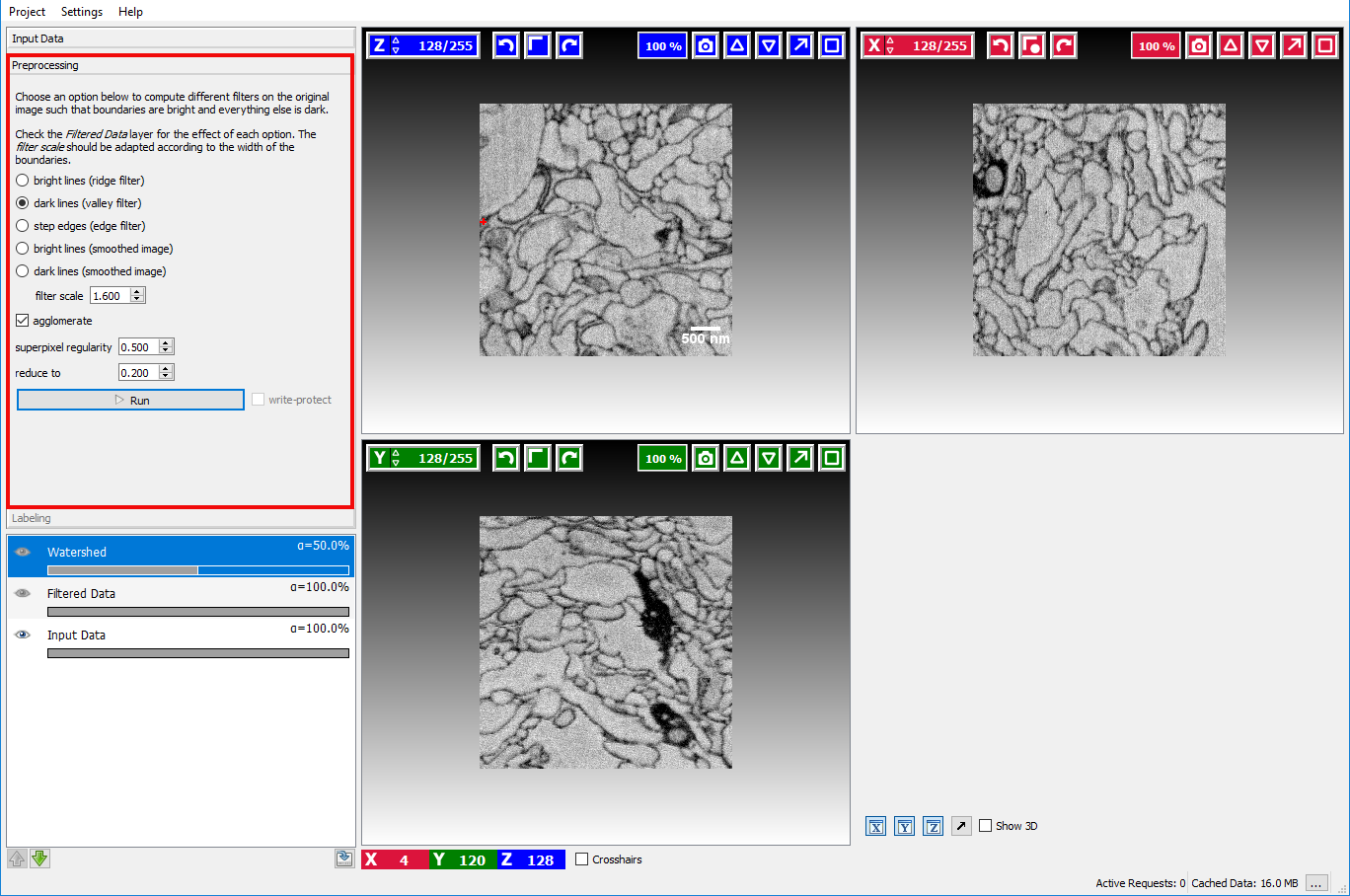
Here the user can select how boundaries are represented in the image.
- Bright lines
- Dark lines
- Step edges: if the boundaries in the image appear as a transition from a bright to a dark region.
- Bright lines (smoothed image): if the loaded image is already a boundary map, where bright pixels correspond to an image boundary.
- Dark lines (smoothed image): if the loaded image is already a boundary map, where dark pixels correspond to an image boundary.
In the example image above, a good boundary choice would clearly be dark lines.
To check if the computed boundaries visually correspond with the edges in the image the visibility of the Filtered Data layer
can be toggled by clicking on the eye icon ( ) in that layer:
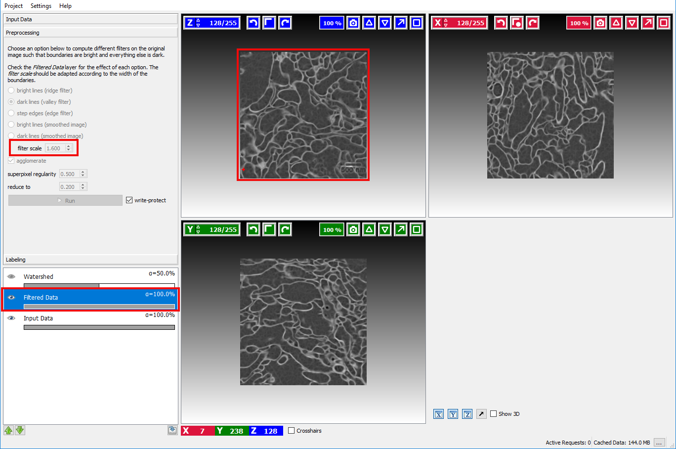
If the boundary map looks too noisy or overly smooth the size of the smoothing kernel needs to be changed with the sigma option. The Filtered Data layer is updated when the user changes the size of the smoothing kernel. This setting should be changed until a satisfactory boundary map is obtained.
When everything looks fine, the user can click on the Run Preprocessing button to calculate a sparse supervoxel graph of the image and boundary map which will speed up segmentation times.
Note: The preprocessing may take a long time depending on the size of the dataset. On a i7 2.4GHz computer a 500×500×500 3D dataset requires 15 minutes of preprocessing.
Interactive Segmentation
After the necessary preprocessing the interactive segmentation of objects in the labeling applet is the next step.
Two different types of seeds exist, Object seeds and Background seeds - per default the background seed receives a higher priority such that the background seed is preferred in the case of ambiguous boundaries.
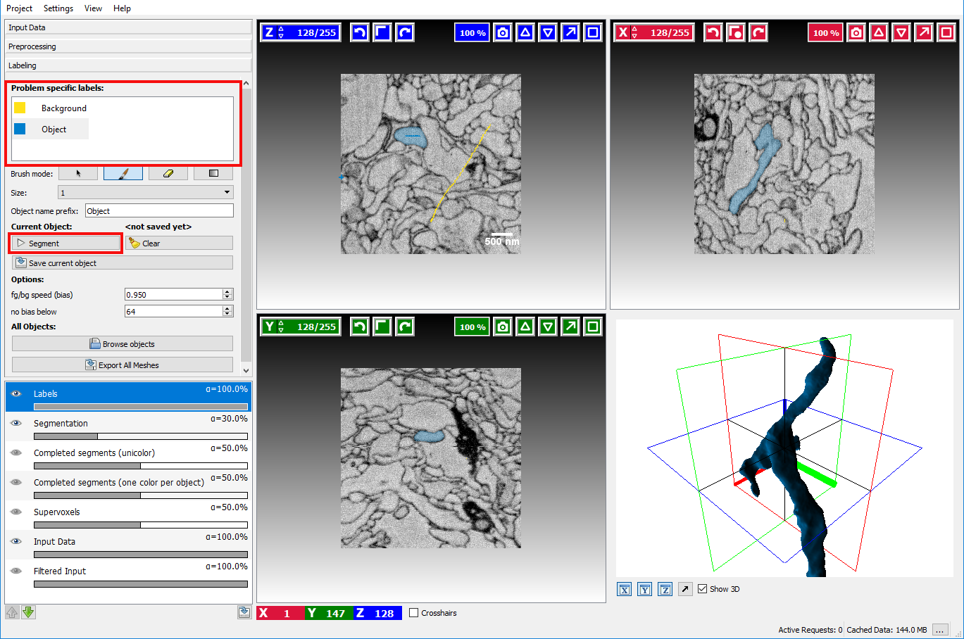
After marking the objects of interest with an object seed and the outside with a background seed the button Segment can be clicked to obtain a seeded watershed segmentation starting from the seeds.
The seeds can be refined by drawing markers, the currently active seed type can be selected on the left side by clicking on the corresponding seed. To erase erroneous markers, the Brush mode (below the seeds) needs to be changed to the eraser to switch back to drawing mode the paint brush item has to be activated again. You can use the Label Explorer to find all existing annotations/seeds.
Additional available interactions include:
- Updating the segmentation: Left click on button Segment
- Erasing a brush stroke: Change brush mode to eraser by clicking on the eraser button
- Window Leveling Change brush mode by clicking on window leveling tool button

- Changing the active seed type: Left Mouse click on seed in the left-hand side seed list.
- Changing the color of a seed type: Right Mouse click on the corresponding seed in the seed list and select Change Color.
- Erasing all markers: Click on the Clear.button next to the segment button.
- Exporting the current segmentation: Right click on the Segmentation Overlay in the overlay widget and select Export.
To learn more about how to navigate the data (**scroll, change slice, enable/disable overlays, change overlay capacity etc. **) please read the Navigation guide.
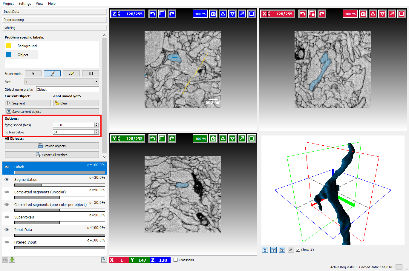
Advanced Options
The seeded watershed algorithm of the module has some advanced options which can be changed to obtain improved segmentations when the default settings are not sufficient.
These additional options described below can be displayed by scrolling down in the labeling applet on the left side.
- BG priority The bias is a parameter the affects how much the background is preferred in comparison to the other labels. A value smaller than 1.0 will lower the detected boundaries for the background seeds. Since the normal seeds still work on the original boundaries the background is preferred in case of ambiguity. Usually, a value of around 0.95 yields good results, but sometimes playing with the parameter is a good way to improve segmentation without additional seeds.
- No bias below The threshold is a value that affects when the BG priority for the background will be applied. Normally the background seed is only preferred when the boundaries are sufficiently strong, i.e. > 64 (the boundaries in the image have values between 0 and 255). Usually, it is not necessary to change this parameter.
Saving and loading segmented objects
Once the user has successfully segmented an object, the result can be stored by clicking on the Save As button. A dialog will pop up that asks for the object name, by default it will be generated from Object name prefix and sequential number:
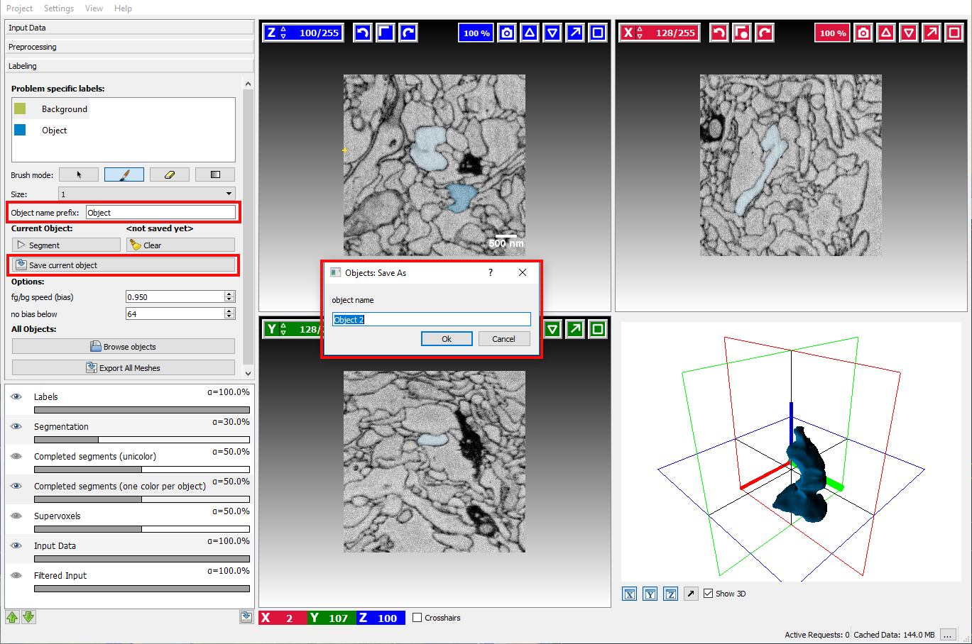
After saving an object, all existing markers will be removed to allow segmenting a new
object from scratch. To see which objects have already been segmented and saved the Completed Segments overlay
can be enabled by clicking on the eye icon () in that layer:
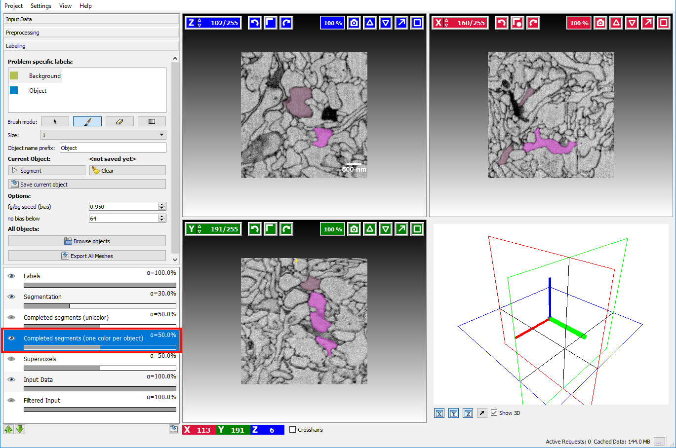
already segmented (and saved) objects will be highlighted to prevent segmenting something twice.
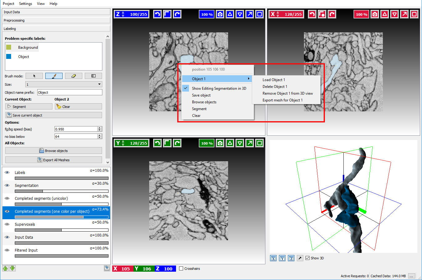
Sometimes it is necessary to refine the segmentation of an already saved object. To do so, click on the Browse objects button and load the corresponding object.
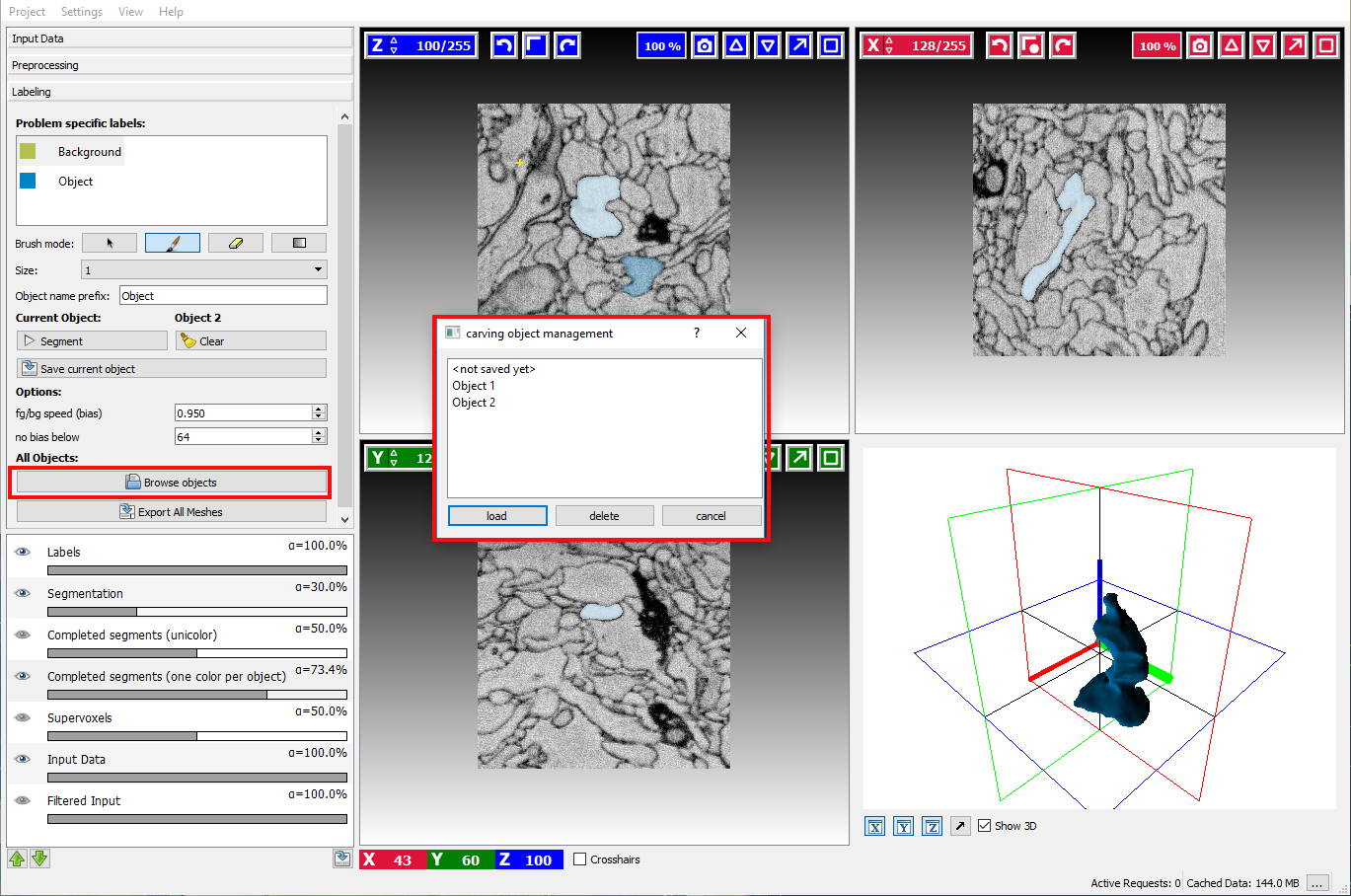
Right-clicking on the highlighted object in Completed segments overlay and navigating to a submenu with object name (in this case it’s “Object 1”) provides the following options:
- Load object name
- Delete object name
- Show 3D object name – will display object in 3D view
- Export mesh for object name – will export mesh of the selected object
Post-processing
Wonderful users of ilastik have created these tools to post-process carving results and made them available for all:
- Neuromorph, for measuring and analyzing the segmented object properties. Featured in
A. Jorstad, B. Nigro, C. Cali, M. Wawrzyniak, P. Fua, G. Knott. “NeuroMorph: A Toolset for the Morphometric Analysis and Visualization of 3D Models Derived from Electron Microscopy Image Stacks.” Neuroinformatics, 2014. - StackObjectCombiner, for glueing together objects from datasets, which were carved blockwise.