Object Classification

Object Classification Demo (3 minutes)

How it works, what it can do

As the name suggests, the object classification workflow aims to classify full objects, based on object-level features and user annotations. An object in this context is a set of pixels that belong to the same instance. Object classification requires a second input besides the usual raw image data: an image that indicates for pixels whether they belong to an object or not, i.e. pixel predictions, a segmentation or a label image. This can be obtained e.g. using the Pixel Classification Workflow. The workflow exists in two variants to handle different types for the second input:

• Object Classification [Inputs: Raw Data, Pixel Prediction Map]
• Object Classification [Inputs: Raw Data, Segmentation]

The combined “Pixel Classification + Object Classification” workflow (found under “Other Workflows”) is primarily intended for demonstration purposes and its use in real projects is discouraged. We instead recommend to use the two workflows separately, exporting probability maps from the Pixel Classification workflow and using them as input for the Object Classification workflow.

Size Limitation:

For object classification, images used in training have to be small enough to fit entirely into your machine’s RAM. However, once you have created a satisfactory classifier using one or more small images (or cutouts from your complete dataset), you can use the “Blockwise Object Classification” feature to run object classification on much larger images (prediction only - no training).

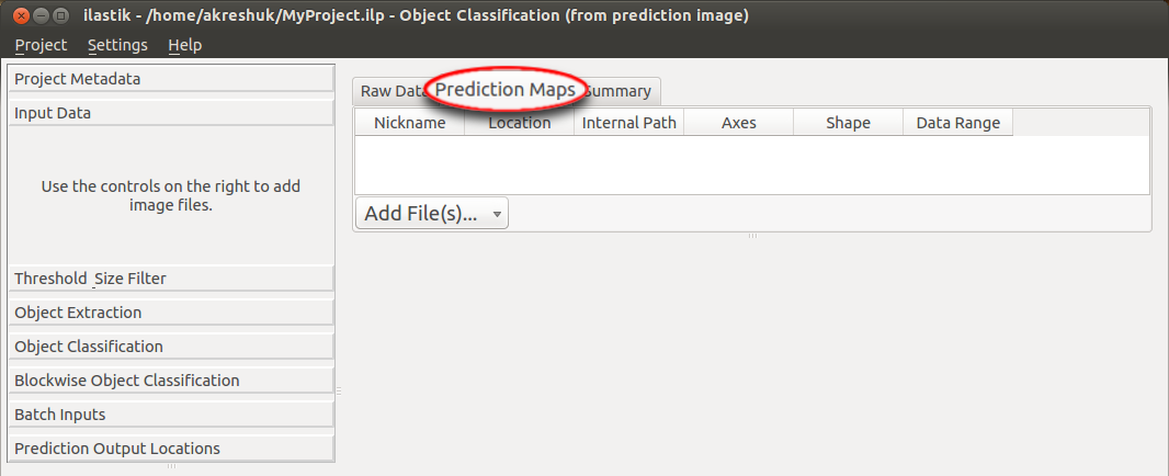
Object Classification [Inputs: Raw Data, Pixel Prediction Map]

You should choose this workflow if you have a probability map, i.e. each pixel value is the pixel’s probability to belong to an object. To obtain a segmentation from this input, the workflow includes a step for thresholding the probabilities. If you use the Pixel Classification workflow to identify objects, we recommend you export the probability maps there and then continue with this object classification workflow.

Load the probability maps in addition to the raw data in the Input Data step:

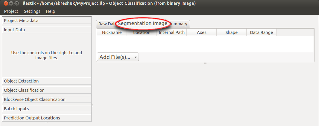
Object Classification [Inputs: Raw Data, Segmentation]

This workflow should be used if you already have a binary segmentation or a label image. Note that background pixels must have the value 0.

The image should be loaded in the data input applet:

From probabilities to a segmentation - “Threshold and Size Filter” applet

This section only applies if you are in the “Object Classification [Inputs: Raw Data, Pixel Prediction Map]” workflow.

Suppose we have a probability map for a 2-class classification, which looks like this:

The basic idea of thresholding is to answer a question for every pixel in an image: is the pixel value larger than the threshold value or not? In ilastik probability maps (result of Pixel Classification) pixel values are in the continuous range from 0.0 to 1.0 in each channel and describe the probability that a pixel belongs into a class. In this applet this continuous range is transferred into a binary one, containing only 0s and 1s (so no values in between) by comparing it to a set threshold.

Note: To see the results of changing the parameter settings in this applet, press the “Apply” button. Also be aware that if you already continued in the workflow, changing parameters here will delete any object labelling you have done.

There are two algorithms you can choose from to threshold your data: Simple and Hysteresis, which can be selected using the “Method” drop down. The most important difference between the two is that hysteresis thresholding makes it possible to separate connected objects.

Both methods share the following parameters:

• Input Channel(s): Select which channel of the probability map contains the objects
• Smooth: Configure sigmas for smoothing the probability map in order to reduce noise. The Gaussian can be anisotropic, i.e. sigmas for all dimensions can be different. This setting is important for very anisotropic data where we recommend not to smooth across the low-resolution axis at all. If you do not want to smooth, just select a very small sigma (like 0.6).
• Threshold value(s): Value to check each pixel/voxel against.
• Size filter: specify the minimum and maximum value (in terms of pixel/voxel counts for 2D/3D, respectively).

For both thresholding methods the end result is shown in the “Final output” layer.

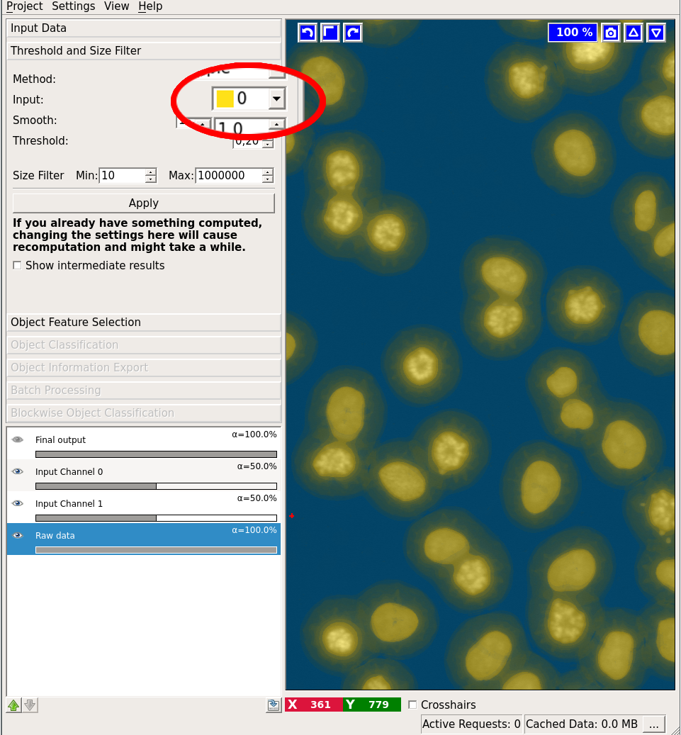
Simple Thresholding

Selecting “Simple” in the Method dropdown will perform regular thresholding at one level, followed by the size filter.

You begin by selecting a channel with the Input dropdown:

Next, you can configure your sigmas for smoothing the probability image. You can check the results of the smoothing operation by first activating the “Show intermediate results” checkbox and then looking at the “Smoothed input” layer:

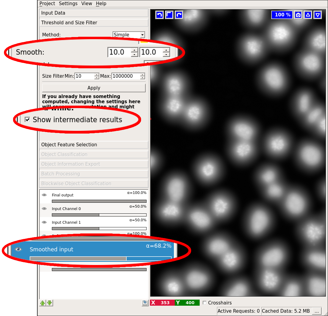
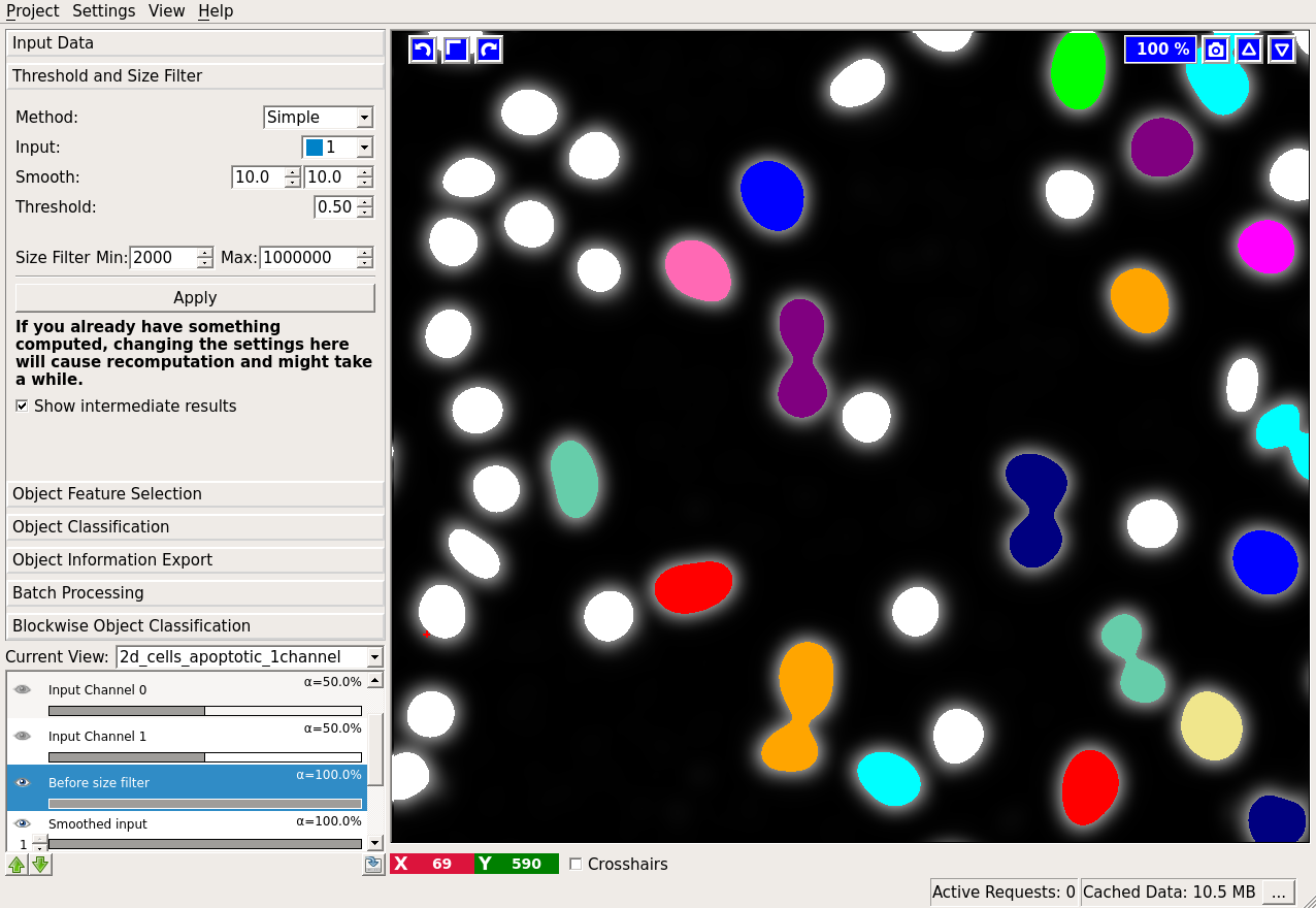
We also provide a view on the thresholded objects before size filtering. This layer is activated by checking the Show intermediate results checkbox. In the example below, the result before size filter is shown in white. After application of the size filter, only the colored objects remain.

Hysteresis Thresholding

By selecting Hysteresis in the method drop-down thresholding is performed at two levels: core, or high threshold, and final, or low threshold. The high threshold is applied first and the resulting objects are filtered by size. These high probability areas act as seeds: For the remaining objects the segmentation is then relaxed to the level of low threshold starting from the seeds. The two levels of thresholding allow to separate the criteria for detection and segmentation of objects and select only objects of very high probability while better preserving their shape. As for the single threshold case, we provide a view on the intermediate results after the application of the high threshold, the size filter and the low threshold. The image below shows the results of the high (detection) threshold after size filter in pink (●) overlayed on the final results of the low (segmentation) threshold multiple colors:

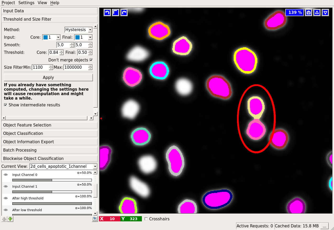
An additional setting is available with Hysteresis Thresholding: Two (or more) seeds (determined by the “core” threshold) might result in the same object when the segmentation is relaxed. With the Don’t merge objects checkbox, you can control this behavior: Checking it, will preserve one object per detection. This is indicated with the red ellipse in the above image: The pink and the yellow object would be merged without checking the Don’t merge objects checkbox.

Now that we have obtained a segmentation, we are ready to proceed to the “Object Feature Selection” applet.

From segmentation to object descriptions - “Object Feature Selection” applet

This applet allows you to choose the features that will be used to classify objects.

The following dialog will appear if you press the “Select features” button:

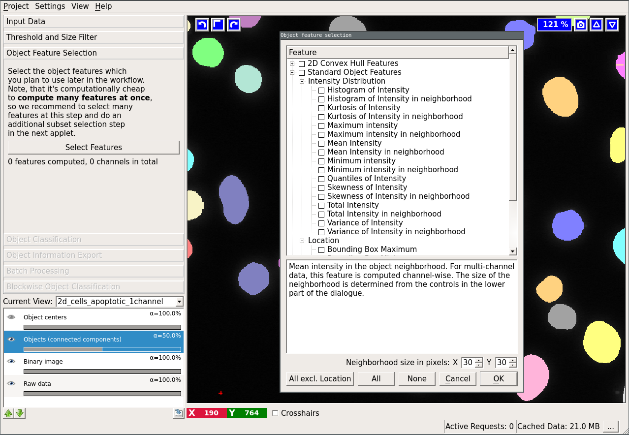
The object feature calculation is plugin-based. Per default ilastik comes with 4 feature plugins:

• “Standard Object Features”
• “Skeleton Features” (2D only)
• “Convex Hull Features”
• “Spherical Texture Features”

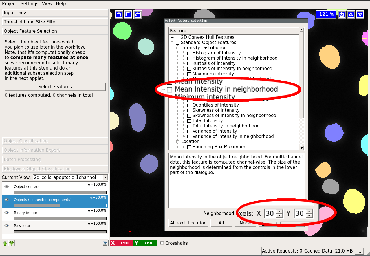
The first three mentioned features are computed by the vigra library. The “Spherical Texture Features” are computed using the SphericalTexture library. An overview of available features can be found in here. The features are subdivided into three groups: “Location”, “Shape”, and “Intensity Distribution”. Location-based features take into account absolute coordinate positions in the image. These are only useful in special cases when the position of the object in the image can be used to infer the object type. Shape-based features extract shape descriptors from the object masks. Lastly, “Intensity Distribution” features operate on image value statistics. You will also notice features, which can be computed “in the neighborhood”. In that case, the neighborhood of the object (specified by the user at the bottom of the dialog) is found by distance transform and the feature is computed for the object itself and for the neighborhood including and excluding the object.

Need more features? Object features are plugin-based and very easy to extend if you know a little Python. A detailed example of a user-defined plugin can be found in the $ILASTIK/examples directory, while this page contains a higher-level description of the few functions you’d have to implement.

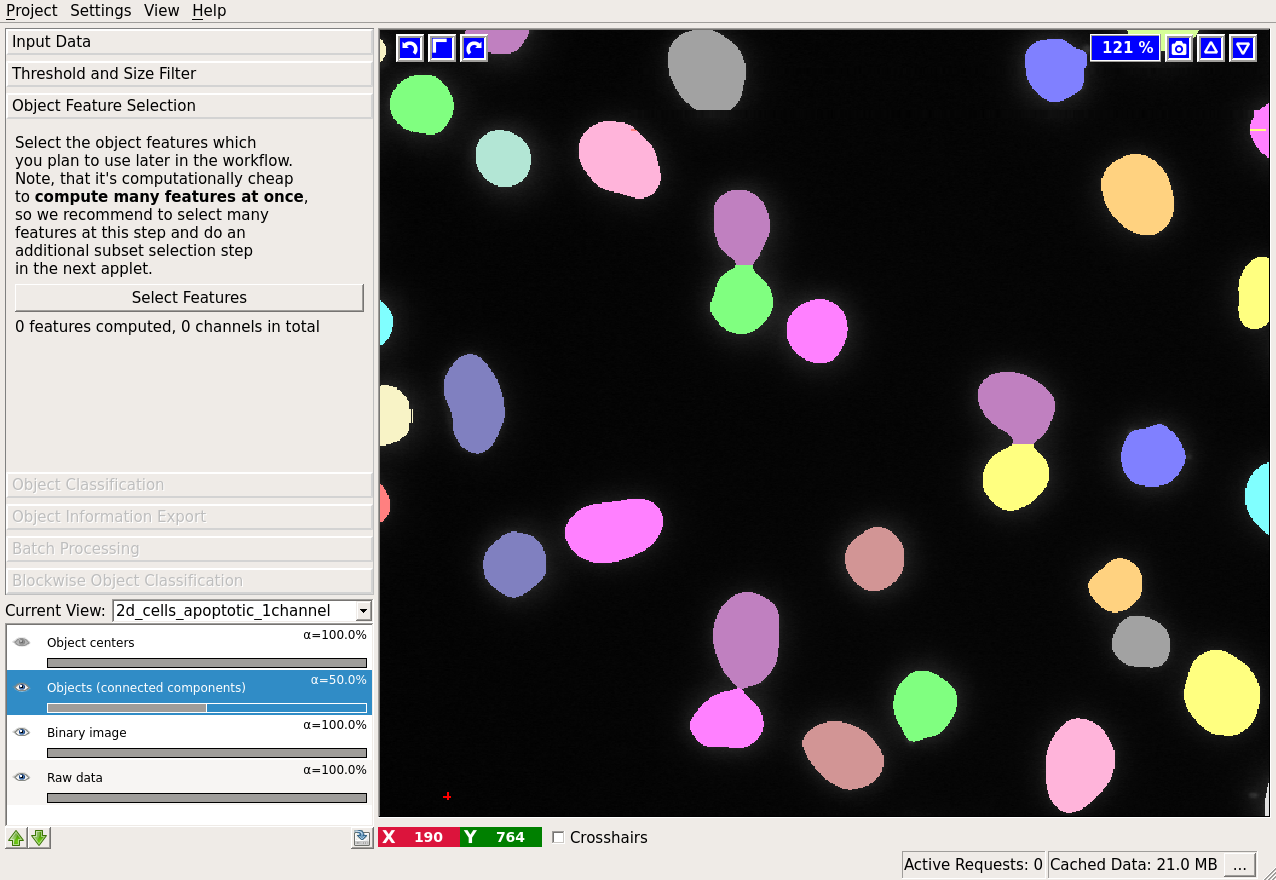
Once you confirm the feature selection, the applet finds the connected components (objects) in the provided binary segmentation image and computes the selected features on them. If you want to inspect the connected components, activate the “Objects (connected components)” layer. For large 3D datasets this step can take quite a while. However, keep in mind that most of the time selecting more features at this step is not more expensive computationally. We therefore recommend that you select all features you think you might try for classification or want to export later and then choose a subset of these features for classification in the next applet.

Prediction for objects - “Object Classification” applet

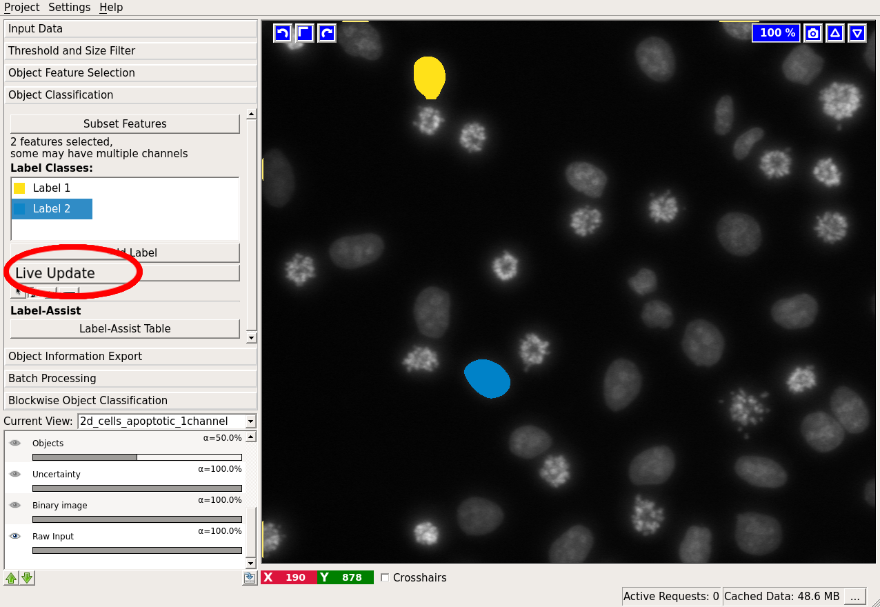
This applet allows you to label the objects and classify them based on the features, computed in the previous applet. Adding labels and changing their color is done the same way as in the Pixel Classification workflow. For a particular example, let us examine the data more closely by activating only the “Raw data” layer (tip: you can toggle between the currently visible layers and only showing the “Raw data” layer by pressing i):

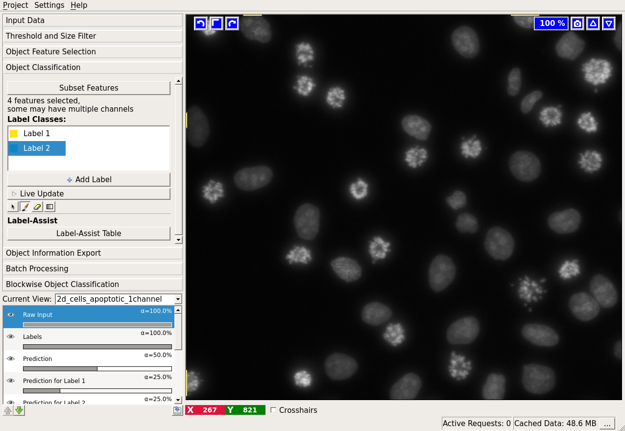
Clearly, two classes of cells are present in the image: one more bright but variable, the other darker and more homogeneous. Hopefully, the two classes can be separated by the grayscale mean and variance in the objects. Let us select these two features. Two labels are already added to the workflow by default. If you need more labels you can click on “Add Label” to do so.

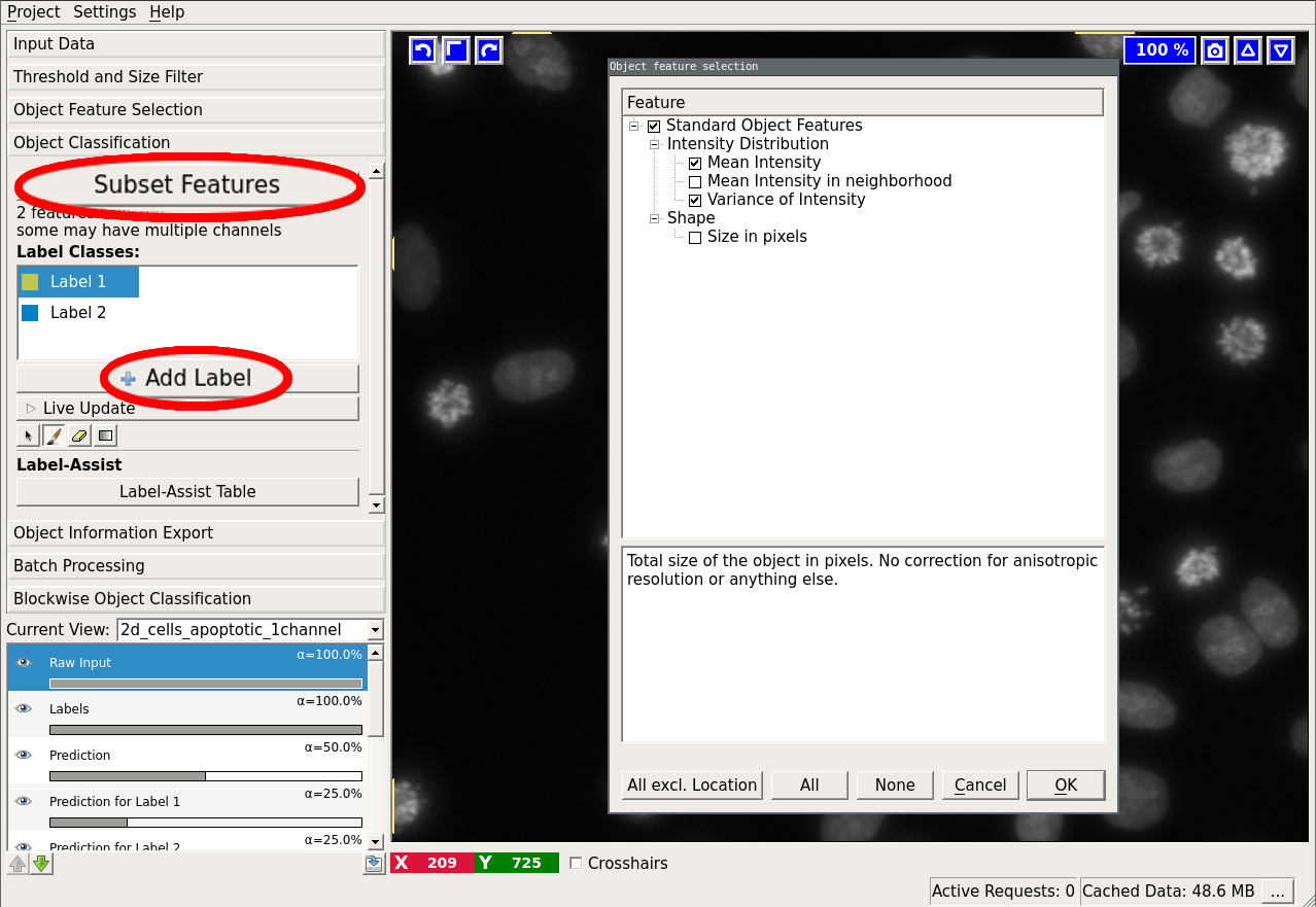
You can subset the features used by the classifier by pressing the “Subset features” button. Note, that the list of features now only contains the few features that were selected in the previous applet. The main purpose for this is to remove features that turn out unhelpful for classification while you are labelling. If you instead go back to Object Feature Selection and remove them, ilastik will recompute the connected components and all features, which can be quite time-consuming. It is also useful if you want to compute and export some features for downstream analysis, even though they should not be used for classification. In that case, you can select all features of interest in the Object Feature Selection applet, and then choose the subset for the classifier here.

To label objects, either simply left-click on them or right-click and select the corresponding option. Right-clicking also allows you to print the object properties in the terminal. To trigger classification, press the “Live Update” button.

If the “Live Update” mode is activated, the prediction is interactive and you can receive immediate feedback on your labels. Let us examine the prediction results:

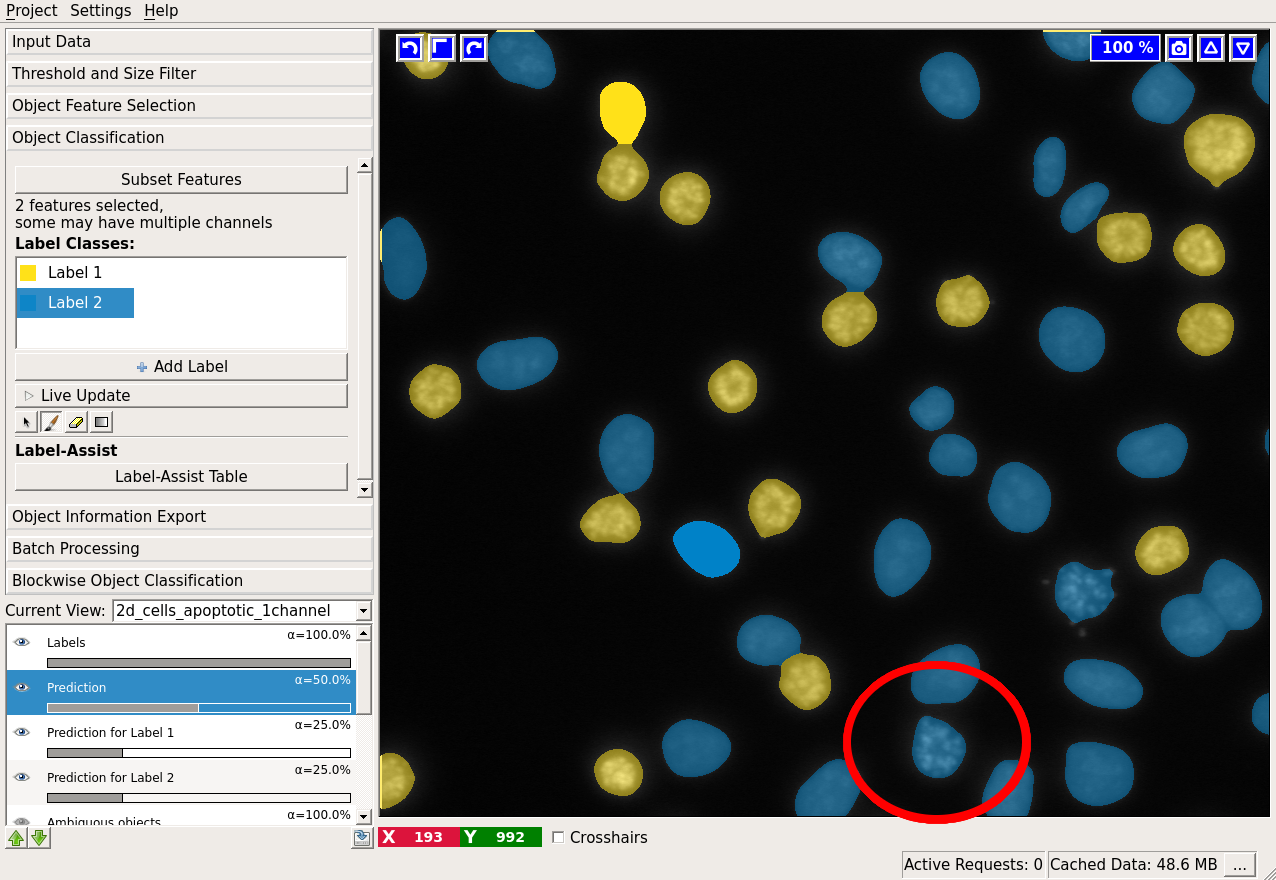
In the low right corner we see a cell (shown by the red ellipse), which was classified as “blue”, while it is most probably “yellow”. Let’s label it “yellow” and check the results again:

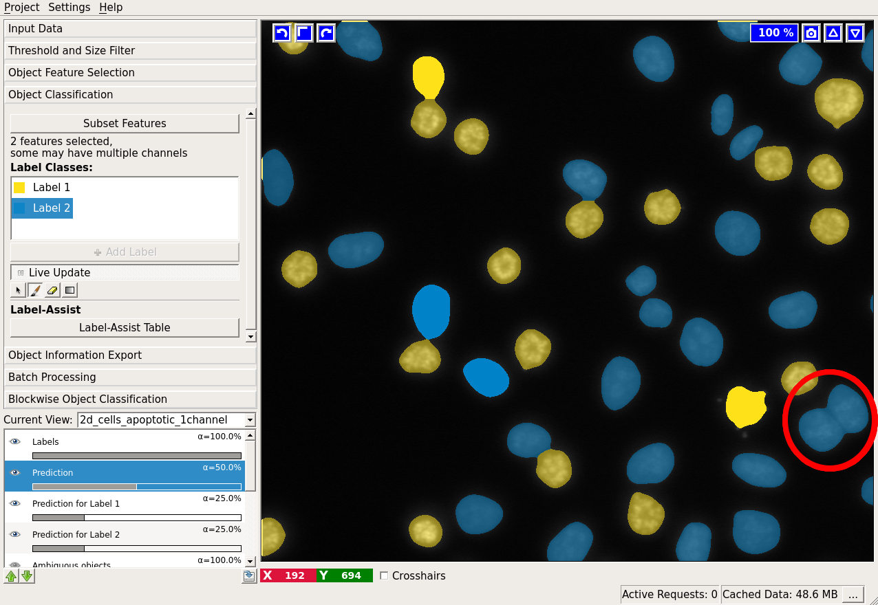
All cells seem to be classified correctly, except one segmentation error, where two cells were erroneously merged (shown by the red ellipse). How could we correct that? We’d have to go back to the thresholding applet, where we performed the segmentation. In the best case, you would have caught this error by examining the thresholding output at the first step. The problem with correcting the segmentation now is that with different thresholds the objects will most probably change shape and thus their features. Besides, some objects might disappear completely, while others appear from the background. Currently, all labels are lost when the threshold is changed!

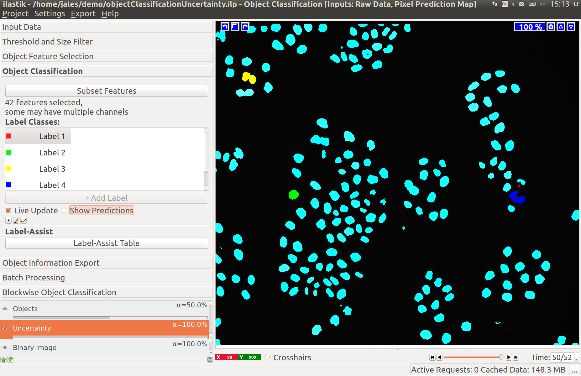
Uncertainty Layer

The Uncertainty layer displays how uncertain the prediction for each object is. As in other workflows, this can be used to identify where the classifier needs more labels to improve the quality of the classification results.

Applying the minimum number of labels for classifying objects containing up to three cells we have a very uncertain classification:

Adding a few more labels reduces the uncertainty for most objects:

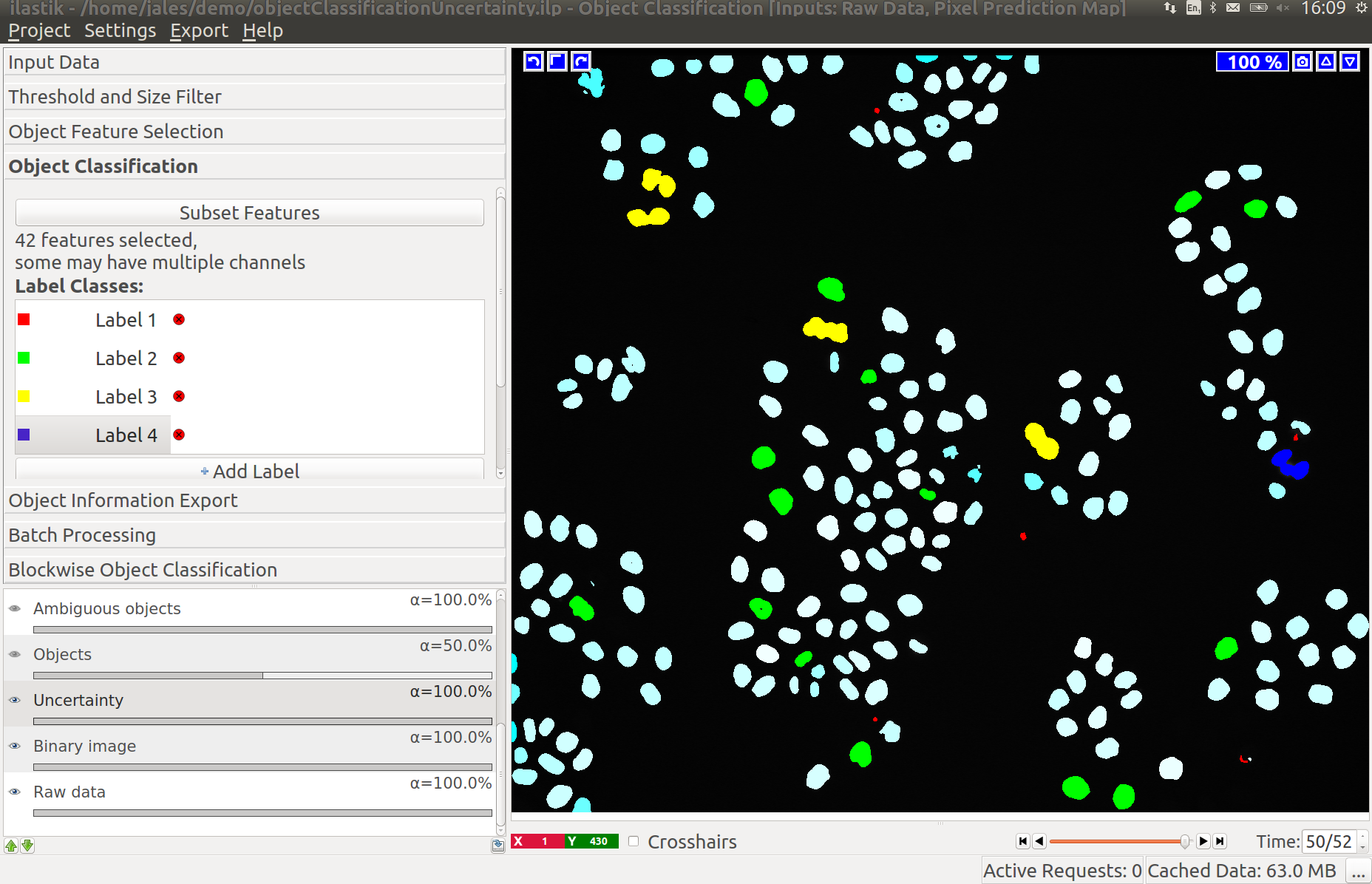
Assuming our labels were correct this will lead to a good object classification:

Export

Regular image exports

In the Export Applet you can export:

• Object Predictions: An image where all pixels belonging to an object have the value of the object’s most probable category (1 for the first label category, 2 for the second, etc.)
• Object Probabilities: A multichannel image with one channel per object (label) class. In each channel, pixels belonging to an object hold the probability value for the respective class.
• Blockwise Object Predictions/Probabilities: Same as above, but perform the computation on the input images in blocks of the size specified in the “Blockwise” applet (see below). This makes it possible to process images that are larger than the machine’s RAM.
• Object Identities: An image where all pixels belonging to an object have the value of the object’s id (1 for the first object, 2 for the second, etc.)

Object feature table export

In addition to the image export, it is also possible to generate a table that encompasses all information about the objects used during classification. To activate this export:

1. Access the table configuration with the Configure Feature Table Export button. See below for more details on the configuration options.
2. Change the file name and choose your preferred format.
3. Choose the features you want to include in the table.
4. Confirm with OK.

Once the table export has been configured, any regular image export (predictions, probabilities) will also generate the table file according to the chosen settings.

The table export can be configured in three sections:

• General: Choose Filename and Format. Note on formats: csv will export a table that can be read with common tools like LibreOffice, or Microsoft Excel. Exporting a table to h5 is most suitable for more involved post-processing, e.g. with Python. In addition to the table data, images of the respective objects can be included in the h5 file, see Settings.
• Features: Select the features to be included in the exported table.
• Settings: Only applicable for h5 export. Per default only the bounding box of each object is exported. A margin can be configured to include context around this bounding box (size in pixels/voxels). Alternatively, it is also possible to include the whole image instead of the individual object images.

HDF5 export format

HDF5 is a flexible cross platform binary data format. Using Python, you can access the data inside the h5 files using the h5py library.

The h5 file contains two items at the root level, images and table. Using h5py, you can access them like a python dictionary:

import h5py
data = h5py.File("path/to/data.h5", "r")
data.keys()
# <KeysViewHDF5 ["images", "table"]>

In the images group you will find a subgroup for each object (identifiable by object_id) which contains two datasets: labeling (cutout of the segmentation showing the object) and raw (cutout of the raw data showing the object).

data["images"].keys()
# <KeysViewHDF5 ["0", "1", "2", "3", ...]>

Access individual the raw and labeling images for each object using the key for the object:

data["images"]["1"].keys()
# <KeysViewHDF5 ["labeling", "raw"]>
data["images"]["1"]["labeling"]
# <HDF5 dataset "labeling": shape (28, 26, 13), type "|u1">
# stored as a numpy array, access the data using numpy indexing:
data["images"]["1"]["labeling"][:]
# image data...

The measurements table is saved as a numpy structured array and holds the selected feature values for each object. The “columns” are saved as dtypes (you can see all column names in your table):

data["table"].dtype.names
#("object_id", "timestep", "Predicted Class" ...)

Individual fields can be accessed by name:

data["table"]["Mean Intensity"]
# array([1551.2393, 1420.5,...], dtype=float32)

Returning a numpy array of Mean Intensity values for all the detected objects. You can access an individual object’s measurements using an index:

data["table"]["Mean Intensity"][0]
# 1551.2393

Returning the Mean Intensity of the first object.

Preparing for large scale prediction - Blockwise Object Classification applet

Segmentation and connected components analysis in the applets above is performed on the whole dataset simultaneously. While these operations and especially the hysteresis thresholding require a lot of RAM, whole image processing is sufficient for most 2D images. However, for large 3D image volumes we have to resort to a different strategy: Traning the classifier on a cutout of the whole image and subsequent blockwise processing of the whole dataset in batch mode. In blockwise processing, the whole dataset is automatically subdivided in a number of blocks that are processed independently. Two parameters control the total size of the blocks:

• block size: Defines size of the block in pixels/voxels in the respective spacial direction. The larger this size, the more RAM will be needed for computation but the image will be subdivided into a smaller number of blocks.
• halo size: Objects might be cut off at the edges of the blocks such that the algorithm does not see the complete object. Mis-classifications are likely in this situation. The halo, with it’s size given in pixels/voxels defines the area/volume around the block that is taken into account in addition to the current block. Choose this parameter to be in the order of the size of the objects.

The Blockwise Object Classification applet allows you to experiment with different block and halo sizes on the data you used in the interactive object prediction. By comparing the “whole image” interactive prediction and blockwise prediction, you can find the optimal parameters for your data. The following example illustrates the process.

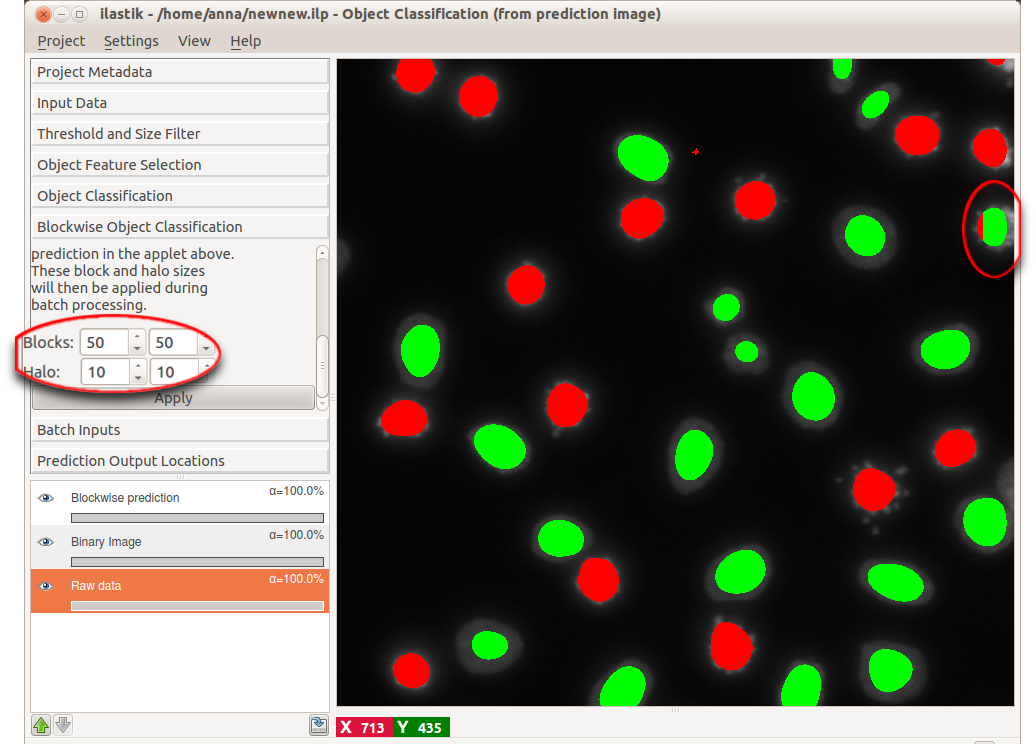In the upper right corner, an object is shown for which the blockwise object classification clearly failed. This object, however, will be predicted correctly if we choose a more reasonable block and halo size. Supposing we found such sizes, let us proceed to batch prediction itself

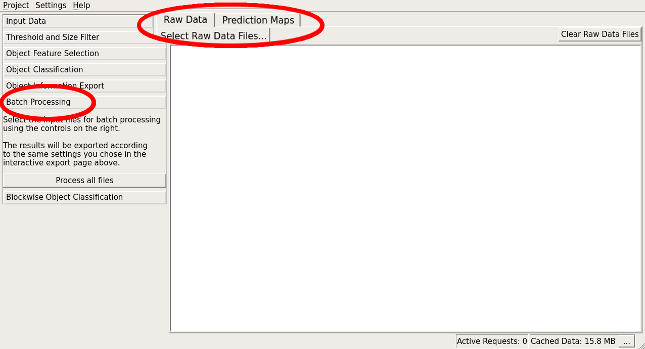
Processing new images in batch mode

After having trained the classifier on one, or a few datasets you can apply it conveniently to a large number of images in the Batch Processing Applet. Note, that for each of the images there, the same export options are applied that are configured in the Export Applet (make sure to use the “magic” placeholders in your output filename there, in order to generate a new result file for every input). Details on all export options can be found on this page These two applets have the same interface and parameters as batch prediction in Pixel Classification workflow. The only difference is that you started the object classification workflow from binary images or prediction images, you’ll have to provide these additional images here as well:

Alternatively you call ilastik without the graphical user interface in headless mode in order to process large numbers of files.